Linear Algebra (I)
Motivation
When I was learning Linear Algebra in University, I found it was hard to understand what would applications of this course. I remember that we learned determinant on Chapter 1, then we learned a lot of other concept such as Rank and EigenValue. I could only memorize one after another theorems without knowing why these happened to appear this way. However, when I was learning matrices from lectures taught by Gilbert Strang, I found every conclusion is so nature that I could easily understand and associate a bunch of concepts with each other. I'd like to conclude what I had learned from him as well as hoping that someone can learn from that.
Why this subject exists?
First of all, what is the origin of linear algebra? Why we make the world increasingly complicated? The truth is that the purpose of mathmatics is to make the world simpler, not the opposite, Linear Algebra as well. For example, we want to solve equations with a lot of variables, the original way is to write all the parameter out: \[\begin{cases} 3x+4y+6z = 0\\\\ 2x+3y+4z = 24\\\\ x+y+z = 15 \end{cases}\]If there are only 3 parameters, the problems is not so hard for us to
handle. But what if there are 100 parameters? When we transfer the
equation to matrices, the outcome becomes so grateful: \[\begin{align}
\begin{bmatrix}
3&4&6\\\\
2&3&4\\\\
1&1&1
\end{bmatrix}
\begin{bmatrix}
x\\\\
y\\\\
z
\end{bmatrix}=\begin{bmatrix}0\\\\24\\\\15\end{bmatrix}
\end{align}\] ### Solve the equation group Now, we try to solve
the problems, our instinction is to draw the three planes, under most
circumstance, there will be a cross point, octave code and the plot is
as followed: 1
2
3
4
5
6
7
8
9
10
11
12
13
14octave:1> x=linspace(-20, 20, 100);
octave:2> [xx, yy] = meshgrid(x,y);
octave:3> z = 15-xx-yy;
octave:4> mesh(xx, yy, z);
octave:5> l = (-3*xx-4*yy)./6;
octave:6> mesh(xx,yy, l);
octave:7> t = (24-(2*xx+3*yy))./4;
octave:8> mesh(xx,yy,z);
octave:9> hold on;
octave:11> mesh(xx,yy,t);
octave:12> mesh(xx,yy,l);
octave:13> xlabel("x")
octave:14> ylabel("y")
octave:15> zlabel("z")
The answer of this equation group is that \[\begin{align} \begin{bmatrix} x\\\\ y\\\\ z \end{bmatrix}=\begin{bmatrix} -18\\\\ 72\\\ -39 \end{bmatrix} \end{align}\]x} \end{align}
Another perspective
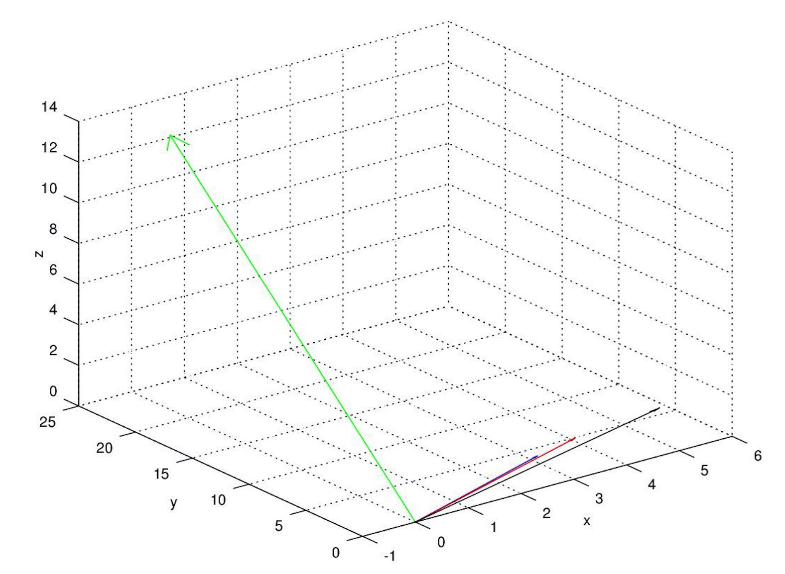
We can find another perspective to solve this equation: see the
equation as a combination of columns, that means: \[\begin{align}
x\*\begin{bmatrix}
3\\\\
2\\\\
1
\end{bmatrix}+y\*
\begin{bmatrix}
4\\\\
3\\\\
1
\end{bmatrix}+z\*
\begin{bmatrix}
6\\\\
4\\\\
1
\end{bmatrix}=
\begin{bmatrix}
0\\\\
24\\\\
15
\end{bmatrix}
\end{align}\] Now, we can acquire the new vector through three
vectors' combination, from the plot blow demonstrates that we need to
find a combination of red&blue&black vectors to generate another
vector(the green one). Obviously, \(x=-18,y=72,z=-39\) is the only solution of
the combination problem. 1
2
3
4
5
6
7
8
9
10
11
12octave:1> a = quiver3(0, 0, 0, 3,2,1);
octave:2> hold on;
octave:3> b = quiver3(0, 0, 0, 4,3,1);
octave:4> c = quiver3(0, 0, 0, 6,4,1);
octave:5> set(b, "Color", "r");
octave:6> set(c, "Color", "k");
octave:7> set(a, "maxheadsize", 0.02);
octave:8> set(b, "maxheadsize", 0.02);
octave:9> set(c, "maxheadsize", 0.02);
octave:10> d = quiver3(0, 0, 0, 0,24,15);
octave:11> set(d, "Color", "g");
octave:12> set(d, "maxheadsize", 0.02);
Step1, calclate z, step2, calclate y, step3, calclate x. We first
leave a variables z alone with an answer in the third equation. Then, we
substitute z to the second equation, and get y. At last we substitute x
and y to the first equation and get x. if we represent above through
matrices language, it is like this: \[\begin{align}
\begin{bmatrix}
3&4&6\\\\
0&1/3&0\\\\
0&0&-1
\end{bmatrix}
\begin{bmatrix}
x\\\\
y\\\\
z
\end{bmatrix}=
\begin{bmatrix}
0\\\\
24\\\\
39
\end{bmatrix}
\end{align}\] The triangle at bottom-left side is all zeros which
ensure we can solve equations one by one. The process is named
back-substitution. ### Additional thinkings But what if the equation
group looks like: \[\begin{align}
\begin{bmatrix}
1&2&3\\\\
1&2&3\\\\
1&2&3
\end{bmatrix}
\begin{bmatrix}
x\\\\
y\\\\
z
\end{bmatrix}=
\begin{bmatrix}
5\\\\
6\\\\
7
\end{bmatrix}
or
\begin{bmatrix}
3&4\\\\
4&5\\\\
5&6\\\\
6&7\\\\
7&9
\end{bmatrix}
\begin{bmatrix}
x\\\\
y
\end{bmatrix}=
\begin{bmatrix}
5\\\\
5\\\\
5\\\\
5\\\\
5
\end{bmatrix}
\end{align}\]
Next time we will talk about LU decomposition and Rank of a matrix.