Linear Regression for Trump
Introduction
In the end of 2016, Trump occupied the presidency. We are always thinking about how he will build the wall between US and Mexico, Today, I'd like to compute how many resources he would cost if he truly began to build the wall using linear regression.
Data
The table below is some basic information about Chinese GreatWall as well as one item about Hadrian's Wall:
| Age | people(1000) | Years | Length(KM) |
|---|---|---|---|
| Qin Dynasty | 300 | 15 | 5000 |
| Han Dynasty | 500 | 100 | 5000 |
| North Northern Dynasties | 1800 | 12 | 2800 |
| Sui Dynasty | 1280 | 30 | 350 |
| Ming Dynasty | 3000 | 40 | 885 |
| Hadrian's Wall | 18 | 14 | 117 |
We use matrices represent the resources and the length of these walls. Each row of \(x\) represents the quantity of (1000 people and year) men and years, and each row of \(y\) denotes the length of walls(KiloMeter)
\[\begin{align} X=\begin{bmatrix} 5000\\ 5000\\ 2800\\ 350\\ 8851\\ 117 \end{bmatrix} y= \begin{bmatrix} 300\*15\\ 500\*100\\ 1800\*12\\ 1280\*30\\ 3000\*40\\ 18\*14 \end{bmatrix} \end{align}\]
Let's draw the picture of these data: 1
2
3
4
5
6
7% octave
X=[5000;5000;2800;350;8851;117];
y=[300\*15;500\*100; 1800\*12;1280\*30;3000\*40; 18\*14];
xlabel("x (km)");
hold on;
ylabel("y (k people year)");
plot(X,y,"ro", "MarkerFaceColor", "b");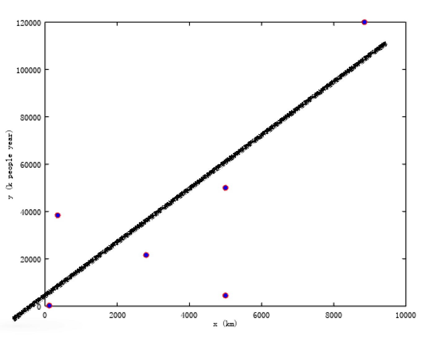 We
hope find a mapping \(x\rightarrow
f(x)\) (\(x\) denotes the length
of walls, \(y\) denotes the cost of
resources)drawing a line as the figure above which meets all data best.
When we encounter new data(e.g. new length of wall), we hope \(f(x)\) will help us find how many resources
will we cost. This is the goal of linear regression.
We
hope find a mapping \(x\rightarrow
f(x)\) (\(x\) denotes the length
of walls, \(y\) denotes the cost of
resources)drawing a line as the figure above which meets all data best.
When we encounter new data(e.g. new length of wall), we hope \(f(x)\) will help us find how many resources
will we cost. This is the goal of linear regression.
Definition
First of all, we assume that the line have the form as followed: \[h\_{\theta}(x)=\theta_0+\theta_1 x_1+\theta_2 x_2 + \cdots + \theta_nx_n\] Specifically, under our circumstance, there is only one \(x\)(the length of walls), then we will have the form as below: \[h\_{\theta}(x)=\theta_0+\theta_1x\] In fact, there are many factor infulence the outcome of the cost of wall besides people and time. Tools we use and the economy as well as terrain where building the wall. if we add these factors, maybe the assumption looks like: \[h\_{\theta}(x)=\theta_0+\theta_1x_1+\theta_2x_2+\theta_3x_2\] \(x_1\)denotes the length of wall, while \(x_2\) and \(x_3\) denote economy and terrian condition respectively. For simplicity, we consider only the length of wall.
In general, we add a \(x_0=1\) to the equation, the we have: \[h\_{\theta}(x)=\theta_0x_0+\theta_1 x_1 + \cdots + \theta_nx_n =\sum\_{i=1}^{n}\theta_ix_i\] If we use matrices represent the equation, then \[\begin{align} \Theta=\begin{bmatrix} \theta_0\\ \theta_1\\ \cdots\\ \theta_n \end{bmatrix} \end{align}\] thus, \[\begin{align} h\_{\theta}(x)=\sum\_{i=1}^{n}\theta_ix_i= \begin{bmatrix} \theta_0\theta_1\cdots\theta_n \end{bmatrix} \begin{bmatrix} x_0\\ x_1\\ \cdots\\ x_n \end{bmatrix} =\Theta^T\overrightarrow{X} \end{align}\] Notice that \(\Theta^T\) is a \(1\times n\) matrices while \(\overrightarrow{X}\) is a \(n\times1\) matrices. We get a real number after multiply two matrices.
Cost Function
We hope find a way to find the best function \(h\_\theta(x)\) fit these data. Notice that
if \(|(h\_\theta(x_i)-y_i)|=0\) for
each \(x\), then the function fit data
absolutely. In practice, if we minimize \(|(h\_\theta(x_i)-y_i)|\), we can find the
best fit to original data. An optional cost function is square cost
function: \[J(\theta)=\frac{1}{2m}\sum\_{i=1}^{m}(h\_\theta(x_i)-y_i)^2\]
As long as we can minimize \(J(\theta)\) with respect to \(\theta\), can we find the best \(\theta\) fit original data. The cost
function looks like as followed: 1
2
3
4
5
6
7
8
9
10
11
12
13
14
15
16
17
18
19
20% octave
m = size(X,1)
XX = [ones(m,1),X];
theta0 = linspace(-100,6000, 100);
theta1 = linspace(-20,36, 100);
l0=length(theta0);
l1=length(theta1);
J_vs = zeros(l0,l1);
for i=1:l0
for j=1:l1
t = [theta0(i); theta1(j)];
J_vs(i,j) = cost(XX, y, t);
end
end
figure;
J_vs = J_vs';
surfc(theta0, theta1, J_vs);
colorbar;
xlabel('\theta_0');
ylabel('\theta_1');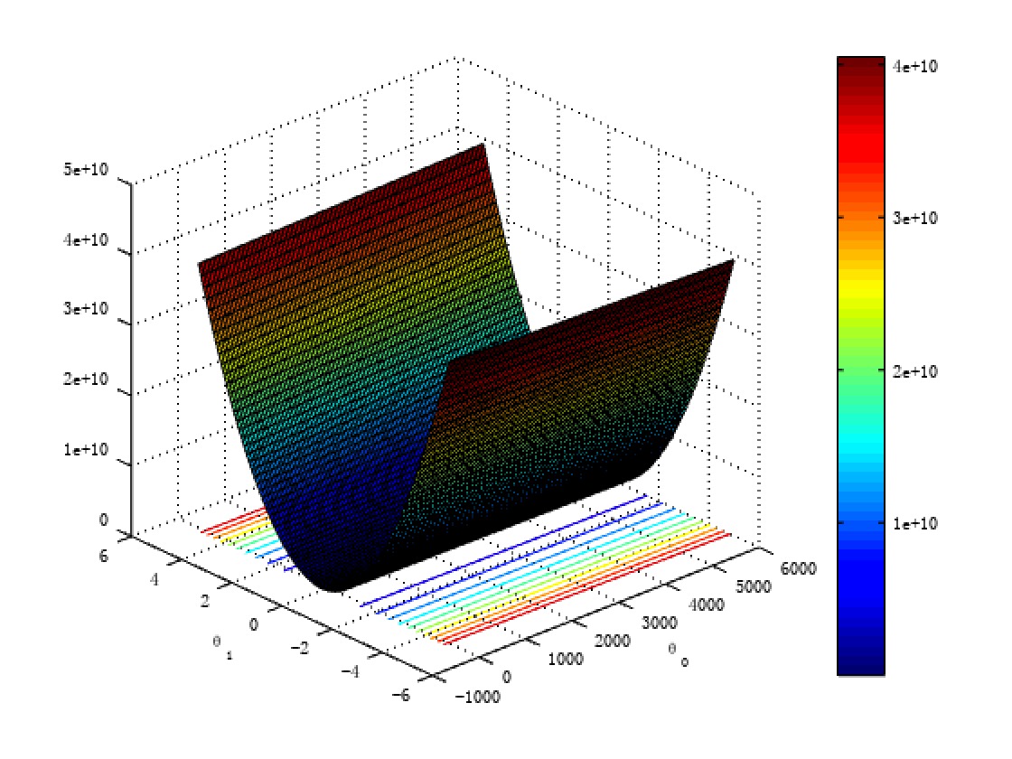
The figure has a bowl shape, and we can find the minimum of it both using matrices approach and gradient descent.
Matrics Solution
Remember that the cost function \(J(\theta)=\frac{1}{2m}\sum\_{i=1}^{m}(h\_\theta(x_i)-y_i)^2\),
It is more convinient if we apply \(J(\theta)\) matrics form, then: \[\begin{align}
J(\theta)=\frac{1}{2m}(h\_\theta(x)-y)^T\cdot(h\_\theta(x)-y)\\
=\frac{1}{2m}(X\Theta-y)^T\cdot(X\Theta-y)
\end{align}\] We can take the derivative of \(J(\theta)\) and let it be \(\overrightarrow{0}\). It is a little
complex if we take the derivative of the last equation about \(J(\theta)\). Let's do the derivation a easy
way, but not a total Matric solution. If we do the derivation on the
sum, we can get: \[\frac{\partial}{\partial\theta_j}J(\theta)=\frac{1}{m}\sum\_{i=1}^m(h\_\theta(x_i)-y_i)x_j\]
Then, \[\begin{align}
\frac{\partial}{\partial\Theta}J(\theta)=
\begin{bmatrix}
\frac{\partial}{\partial\theta_1}J(\theta)\\
\frac{\partial}{\partial\theta_2}J(\theta)\\
\frac{\partial}{\partial\theta_3}J(\theta)\\
\cdots\\
\frac{\partial}{\partial\theta_n}J(\theta)
\end{bmatrix}=\overrightarrow{0}
\end{align}\] Now, we transfer the sum into matrices form: \[\frac{\partial}{\partial\Theta}J(\theta)=X^T(X\Theta-y)=X^TX\Theta-X^Ty=\overrightarrow{0}\]
thus, we can get the solution of \(\Theta\): \[\Theta=(X^TX)^{(-1)}X^Ty\] Let's look at
the solution of Matrices: 1
2
3
4
5
6
7
8
9% octave
xlabel("x (km)");
hold on;
ylabel("y (k people year)");
plot(X,y,"ro", "MarkerFaceColor", "b");
a=linspace(0,10000,100);
t = pinv(XX'*XX)*XX'*y;
b=t'*[ones(1, length(a)); a];
plot(a,b);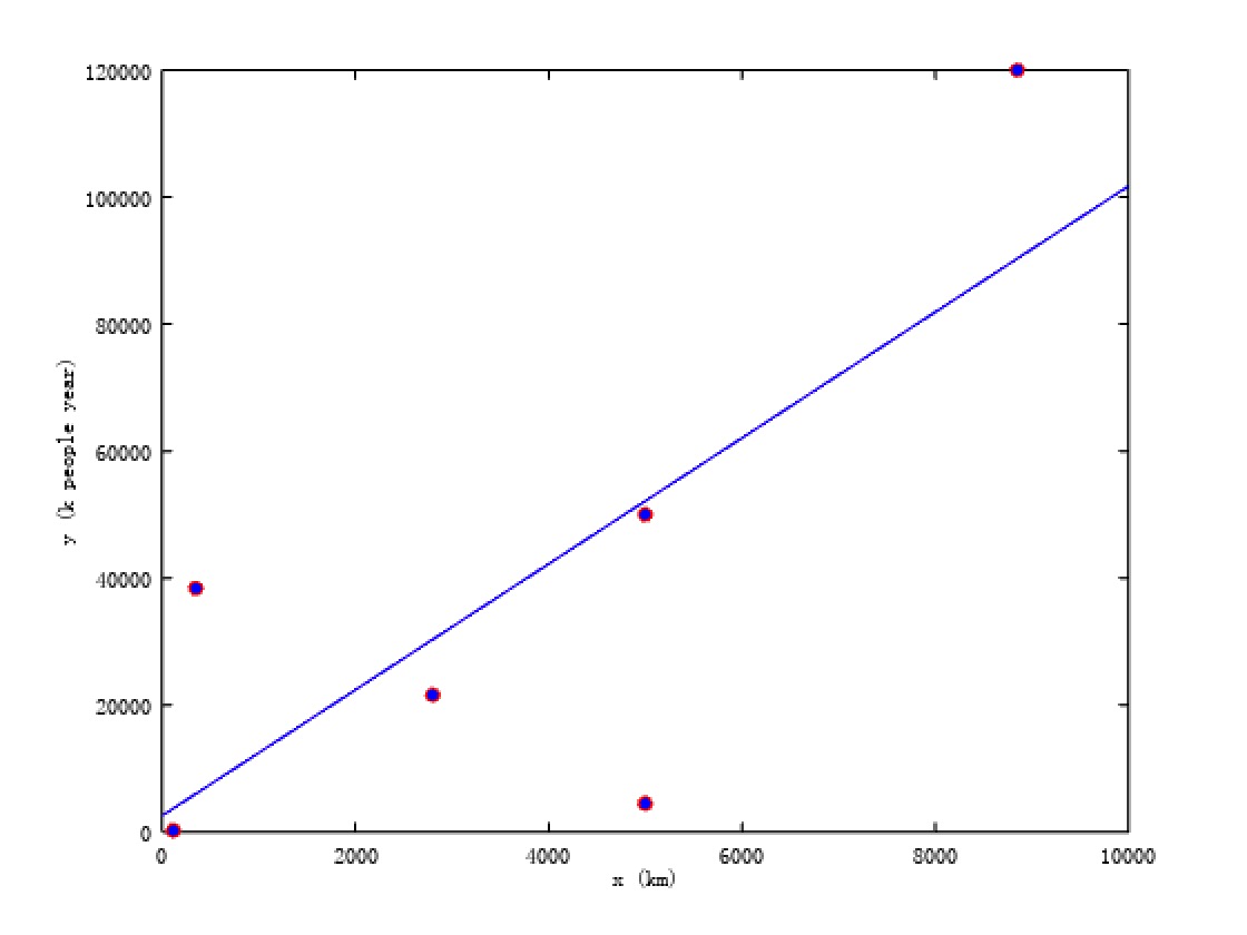
And \(\theta_0\) and \(\theta_1\) is as followed: \[\begin{align}
\Theta=\begin{bmatrix}
2573\\
9.9\\
\end{bmatrix}
\end{align}\] That means \(h\_\theta(x)=2573+9.9x\), Right Now we
subsitute 3169(km) for \(x\): \[h\_\theta(3169)=2573+9.9\*3169=33946(k\ people\
year)\] In other word, Donald Trump need 3,394,600 people
continously build 10 years in order to finish the GreatWall between US
and Mexico. Surely he can stimulate 33,946,000 people, it only take him
one year to finished the wall. ### Gradient Descent Solution Let's look
at the cost function one more time. If we first choose a random \(\Theta\), say we have \(\theta_0\&\theta_1\) located in point
1. Assume you stand at ponit 1, you want to find a way to go down the
vally. Surely you can not see the land-form completely. But you can look
around at point 1 and find a steepest direction, then you go that way a
baby step. Right now, you are at point 2 after the first step. You do
the same find a steepest direction and make another baby step. After
several steps, you are now standing at point 5. When you are looking
around you find that where you are standing is almost flat. Now we can
stop the iteration, and we have found a reasonable \(\Theta\) which makes the \(J(\theta)\) has a minmum value. 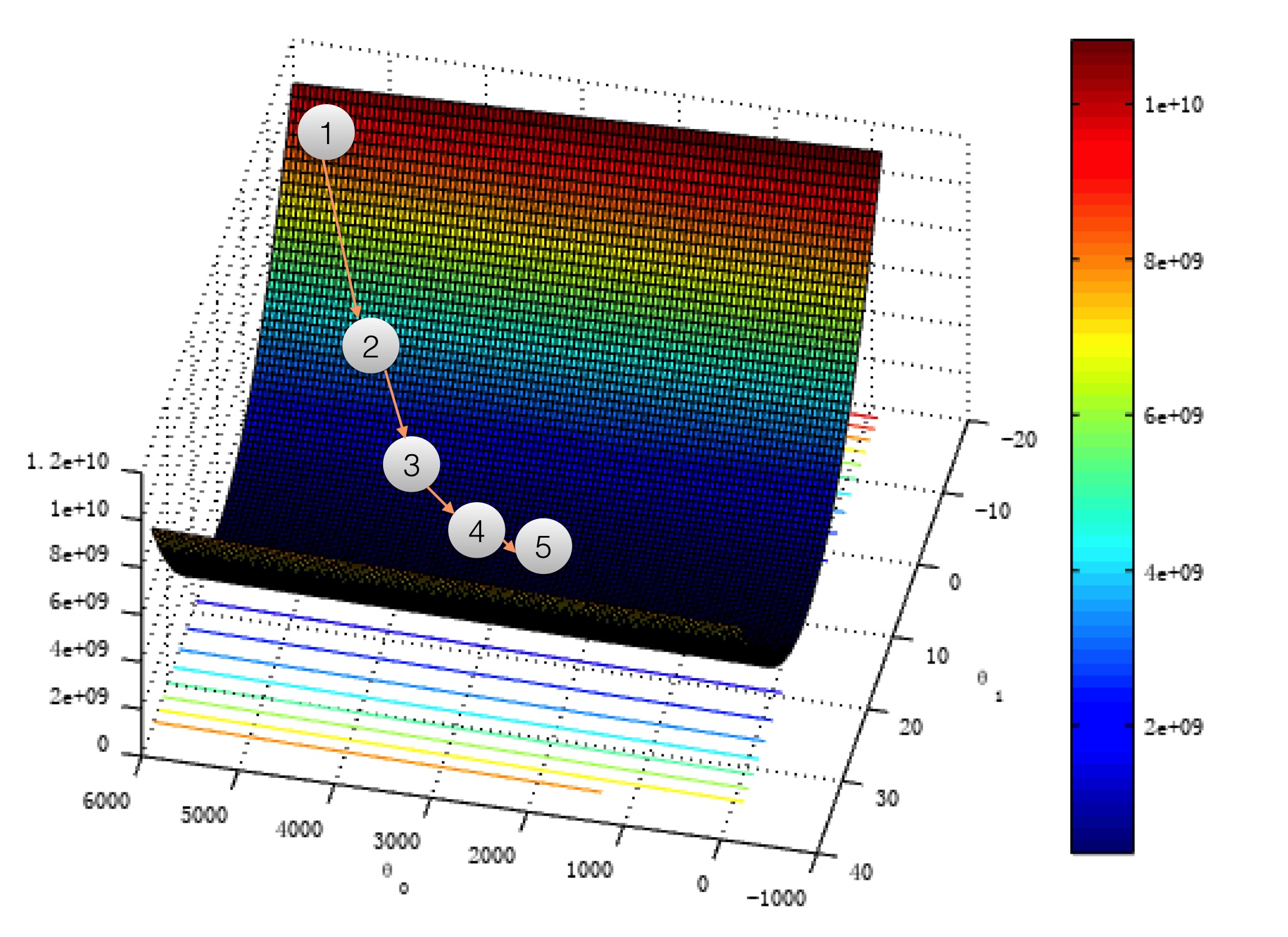 What I described is a method named Gradient Descent which is very easy
way to find minima of \(J(\theta)\).
The step is as followed:
What I described is a method named Gradient Descent which is very easy
way to find minima of \(J(\theta)\).
The step is as followed:
- Find a reasonable cost function J().
- Take the partial derivative of \(J(\theta)\) for each \(\theta_j\)
- Choose a moderate \(\alpha\) to constrain the step size.
- Take a baby step, the direction is from the derivative and the size is determined by derivative and parameter \(alpha\)
- update the value of \(\Theta\), check if we find the minimum. If not, return to the step 4, otherwise, stop the algo
Concretely, the algorithm using octave is listed below: 1
2
3
4
5
6% octave: The derivative function
function g = gradient(X, y, theta)
m = size(X,1);
hx = X*theta;
g = (1/m)*X'*(hx-y);
end1
2
3
4
5
6
7% octave: I just take 100 steps without checking when to stop.
theta=[0;0];
alpha=0.00000003
for i=1:100
g = gradient(XX,y,theta);
theta = theta - alpha*g
end
Appendix
1 | % octave --cost function:cost.m |