A Tutorial on Singular Value Decomposition

发表于 2017-05-01 分类于 Alogorithm

Preface

Under some circumstance, we want to compress data to save storage space. For example, when iPhone7 was released, many were trapped in a dilemma: Should I buy a 32G iPhone without enough free space or that of 128G with a lot of storage being wasted? I had been trapped in such dilemma indeed. I still remember that I only had 8G storage totally when I was using my first Android phone. What annoyed me most was my thousands of photos. Well, I confess that I was being always a mad picture taker. I knew that there were some technique which could compress a picture through reducing pixel. However, it is not enough, because, as you know, in some arbitrary position in a picture, we can tell that the picture share the same color. An extreme Example: if we have a pure color picture, what we just need know is the RGB value and the size, then reproducing the picture is done without extra effort. What I was dreaming is done perfectly by Singular Value Decomposition(SVD).

Introduction

Before SVD, in this article, I will introduce some mathmatical concepts in the first place which cover Linear transformation and EigenVector&EigenValue. This Background knowledge is meant to make SVD straightforward. You can skip if you are familar with this knowledge.

Linear transformation

Given a matrice $A$ and vector $\vec{x}$ , we want to compute the mulplication of $A$ and $\vec{x}$

$\vec{x} = (\begin{matrix} 1 \\ 3 \end{matrix}) A = (\begin{matrix} 2 & 1 \\ - 1 & 1 \end{matrix}) \vec{y} = A \vec{x}$

But when we do this multiplication, what happens? Acutually, when we multiply $A$ and $\vec{x}$ , we are changing the coordinate axes of the vector $x$ to another new axes. Begin with a simpler example, we let

$A = (\begin{matrix} 1 & 0 \\ 0 & 1 \end{matrix})$

then we have $A \vec{x} = (\begin{matrix} 1 & 0 \\ 0 & 1 \end{matrix}) (\begin{matrix} 1 \\ 3 \end{matrix}) = (\begin{matrix} 1 \\ 3 \end{matrix})$

You may have noticed that we can always get the same $\vec{x}$ after left multiply by A. In this case, we use coordinate axes $i = (\begin{matrix} 1 \\ 0 \end{matrix})$ and $j = (\begin{matrix} 0 \\ 1 \end{matrix})$ as the figure below demonstrated. That is, if we want to represent $(\begin{matrix} 1 \\ 3 \end{matrix})$ under the coordination, we can calculate the transformation as followed:

$\begin{array}{r} A \vec{x} = 1 \cdot i + 3 \cdot j = 1 \cdot (\begin{array}{c} 1 \\ 0 \end{array}) + 3 \cdot (\begin{array}{c} 0 \\ 1 \end{array}) = (\begin{array}{c} 1 \\ 3 \end{array}) \end{array}$

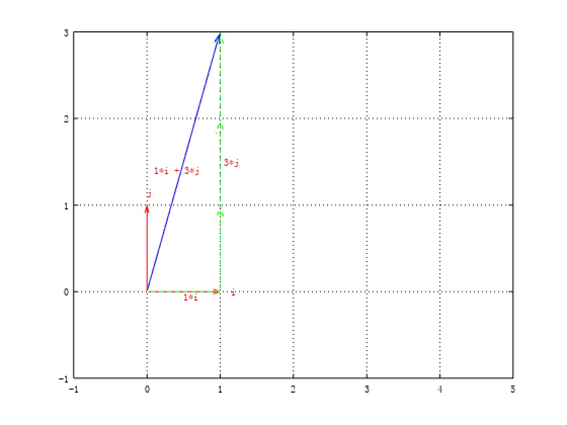
As we know, we can put a vector to anywhere in space, and if we want to calculate sum of two vectors, the simplest way is to connect the to vector from one's head to the other's tail. Our example, we compute $A \vec{x}$ means add two vector(green imaginary lines) up. And the answer is still $(\begin{matrix} 1 \\ 3 \end{matrix})$ .

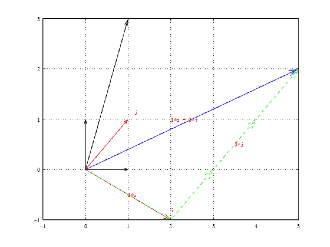
Now we change $i = (\begin{matrix} 2 \\ - 1 \end{matrix})$ and $j = (\begin{matrix} 1 \\ 1 \end{matrix})$ as the coordinate axes(the red vectors), which means $A = (\begin{matrix} 2 & 1 \\ - 1 & 1 \end{matrix})$ . I put vectors(black ones) to this figure as well. We can see what happens when we change a new coordinate axes.

First of all, we multiply $j$ by $3$ and $i$ by 1. Then we move vector j and let the head of $i$ connect the tail of $3 \cdot j$ . We can now find what is the coordination of $1 \cdot i + 3 \cdot j$ (the blue one). We now verify the result using mutiplication of $A$ and $\vec{x}$ :

$A \vec{x} = (\begin{matrix} 2 & 1 \\ - 1 & 1 \end{matrix}) (\begin{matrix} 1 \\ 3 \end{matrix}) = 1 \cdot (\begin{matrix} 2 \\ - 1 \end{matrix}) + 3 \cdot (\begin{matrix} 1 \\ 1 \end{matrix}) = (\begin{matrix} 5 \\ 2 \end{matrix})$

Here, you can imagine that matrice $A$ is just like a function $f (x) \to y$ , when you subsitute $x$ , we get the exact $y$ using the principle $f (x) \to y$ . In fact, the multiplication is tranform the vector from one coordination to another.

Exercise

$A = (\begin{matrix} 1 & 2 \\ 3 & 4 \end{matrix})$ , draw the picture to stretch and rotate $x = (\begin{matrix} 1 \\ 3 \end{matrix})$ .
Find a $A$ matrix to rotate $\vec{x} = (\begin{matrix} 1 \\ 3 \end{matrix})$ to $90^{\circ}$ and $180^{\circ}$ .
what if $A = (\begin{matrix} 1 & 2 \\ 2 & 4 \end{matrix})$ .

EigenVector and EigenValue

EigenVector and EigenValue is an extremely important concept in linear algebra, and is commonly used everywhere including SVD we are talking today. However, many do not know how to interpret it. In fact, EigenVector and EigenValue is very easy as long as we know about what is linear transformation.

A Problem

Before start, let's take a look at a question: if we want to multiply matrices for 1000 times, how to calculate effectively? $A A A \dots A = (\begin{matrix} 3 & 1 \\ 0 & 2 \end{matrix}) (\begin{matrix} 3 & 1 \\ 0 & 2 \end{matrix}) (\begin{matrix} 3 & 1 \\ 0 & 2 \end{matrix}) \dots (\begin{matrix} 3 & 1 \\ 0 & 2 \end{matrix}) = \prod_{i = 1}^{1000} (\begin{matrix} 3 & 1 \\ 0 & 2 \end{matrix})$

Intuition

Last section, we have talked that if we multiply a vector by a matrix $A$ , means that we use $A$ to stretch and rotate the vector in order to represent the vector in a new coordinate axes. However, there are some vectors for $A$ , they can only be stretched but can not be rotated. Assume $A = (\begin{matrix} 3 & 1 \\ 0 & 2 \end{matrix})$ , let $\vec{x} = (\begin{matrix} 1 \\ - 1 \end{matrix})$ . When we multiply $A$ and $\vec{x}$

$A \vec{x} = (\begin{matrix} 3 & 1 \\ 0 & 2 \end{matrix}) (\begin{matrix} 1 \\ - 1 \end{matrix}) = (\begin{matrix} 2 \\ - 2 \end{matrix}) = 2 \cdot (\begin{matrix} 1 \\ - 1 \end{matrix})$

It turns out we can choose any vector along $\vec{x}$ , the outcome is the same, for example:

$A \vec{x} = (\begin{matrix} 3 & 1 \\ 0 & 2 \end{matrix}) (\begin{matrix} - 3 \\ 3 \end{matrix}) = (\begin{matrix} - 6 \\ - 6 \end{matrix}) = 2 \cdot (\begin{matrix} - 3 \\ 3 \end{matrix})$

We name vectors like $(\begin{matrix} - 3 \\ 3 \end{matrix})$ and $(\begin{matrix} 1 \\ - 1 \end{matrix})$ EigenVectors and 2 the conresponse EigenValues. In practice, we usually choose unit eigenvectors(length equals to 1) given that there are innumerable EigenVectors along the line.

I won't cover how to compute these vectors and vaules and just list the answer as followed

$\begin{aligned} (\begin{array}{c} 3 & 1 \\ 0 & 2 \end{array}) (\begin{array}{c} - 1 / \sqrt{(} 2) \\ 1 / \sqrt{(} 2) \end{array}) = 2 (\begin{array}{c} - 1 / \sqrt{(} 2) \\ 1 / \sqrt{(} 2) \end{array}) \vec{x_{1}} = (\begin{array}{c} - 1 / \sqrt{(} 2) \\ 1 / \sqrt{(} 2) \end{array}) & λ_{1} = 2 \\ (\begin{array}{c} 3 & 1 \\ 0 & 2 \end{array}) (\begin{array}{c} 1 \\ 0 \end{array}) = 3 (\begin{array}{c} 1 \\ 0 \end{array}) \vec{x_{2}} = (\begin{array}{c} 1 \\ 0 \end{array}) & λ_{2} = 3 \end{aligned}$ Notice that $| \vec{x_{1}} | = 1$ and $| \vec{x_{2}} | = 1$ #### EigenValue Decomposition If we put two EigenVectors and corresponding EigenValues together, we can get the following equation: $A Q = (\begin{matrix} 3 & 1 \\ 0 & 2 \end{matrix}) (\begin{matrix} - 1 / \sqrt{(} 2) & 1 \\ 1 / \sqrt{(} 2) & 0 \end{matrix}) = (\begin{matrix} - 1 / \sqrt{(} 2) & 1 \\ 1 / \sqrt{(} 2) & 0 \end{matrix}) (\begin{matrix} 2 & 0 \\ 0 & 3 \end{matrix}) = Q Λ$ Then we have $A Q = Q Λ$ , the conclusion is still right if we introduce more dimensions, that is $\begin{array}{r} A \vec{x_{1}} = λ \vec{x_{1}} \\ A \vec{x_{2}} = λ \vec{x_{2}} \\ ⋮ \\ A \vec{x_{k}} = λ \vec{x_{k}} \end{array}$

$Q = (\begin{matrix} x_{11} & x_{21} & \dots x_{k 1} \\ x_{12} & x_{22} & \dots x_{k 2} \\ ⋮ \\ x_{1 m} & x_{22} & \dots x_{k m} \end{matrix}) Λ = (\begin{matrix} λ_{1} & 0 & \dots & 0 \\ 0 & λ_{2} & \dots & 0 \\ ⋮ & ⋮ & ⋱ \\ 0 & \dots & \dots & λ_{k} \end{matrix})$

If we do something on the equation $A Q = Q Λ$ , then we have: $A Q Q^{- 1} = A = Q Λ Q^{- 1}$ It is EigenVaule Decomposition. #### Resolution Now, Let's look at the question in the beginning of this section $\begin{aligned} A A A \dots A & = (\begin{array}{c} 3 & 1 \\ 0 & 2 \end{array}) (\begin{array}{c} 3 & 1 \\ 0 & 2 \end{array}) (\begin{array}{c} 3 & 1 \\ 0 & 2 \end{array}) \dots (\begin{array}{c} 3 & 1 \\ 0 & 2 \end{array}) = \prod_{i = 1}^{1000} (\begin{array}{c} 3 & 1 \\ 0 & 2 \end{array}) \\ A A A \dots A & = Q Λ Q^{- 1} Q Λ Q^{- 1} Q Λ Q^{- 1} \dots Q Λ Q^{- 1} = Q \prod_{i = 1}^{1000} (\begin{array}{c} 3 & 1 \\ 0 & 2 \end{array}) Q^{- 1} \\ A A A \dots A & = Q Λ Λ \dots Λ Q^{- 1} = Q (\begin{array}{c} 2^{1000} & 0 \\ 0 & 3^{1000} \end{array}) Q^{- 1} \end{aligned}$ The calculation is extremely simple using EVD.

Exercise

Research how to compute EigenVectors and EigenValues, then compute $(\begin{matrix} 1 & 2 & 3 \\ 4 & 5 & 6 \\ 7 & 8 & 9 \end{matrix})$ .
Think about the decisive factor affects how many EigenValues we can get.

Singular Value Decompositon

Notice that EigenVector Decomposition is applied to decompose square matrices. Is there any approach to decompose non-square matrices? The answer is a YES, and the name is Singular Value Decompositon.

Intuition

First of all, let's take a look at what SVD looks like 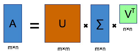From the picture, we can find that matrice $A$ is decomposed to 3 components: $U$ , $Σ$ and $V^{T}$ . $U$ and $V^{T}$ are both sqaure matrices and $Σ$ has the same size as $A$ . Still, I want to emphasize that $U$ and $V^{T}$ are both unitary matrix, which means the Determinant of $U$ and $V^{T}$ is 1 and $U^{T} = U^{- 1} V^{T} = V^{- 1}$ .

Deduction

In the Linear Transformation section, we can transform a vector to another coordinate axes. Assume you have a non-square matrice, and you want to transform A from vectors $V = (\vec{v_{1}}, \vec{v_{2}}, \dots, \vec{v_{n}})^{T}$ to antoher coordinate axes which is $U = (\vec{u_{1}}, \vec{u_{2}}, \dots, \vec{u_{n}})^{T}$ , the thing is, $\vec{v_{i}}$ and $\vec{u_{i}}$ have unit length, and all directions are perpendicular, that is, each of $\vec{v_{i}}$ are at right angles to other $\vec{v_{j}}$ , we name such matrices as orthogonal matrices. In addition, I need add a factor $Σ = (σ_{1}, σ_{2}, σ_{3}, \dots, σ_{n})$ which represent the times of each direction of $\vec{u_{i}}$ , i.e., We need transform A from $V = (\vec{v_{1}}, \vec{v_{2}}, \dots, \vec{v_{n}})^{T}$ to $(σ_{1} \vec{u_{1}}, σ_{2} \vec{u_{2}}, σ_{3} \vec{u_{3}}, . . . σ_{n} \vec{u_{n}})^{T}$ . From the picture below we can find that we want to transform from the circle coordinate axes to the ellipse axes. 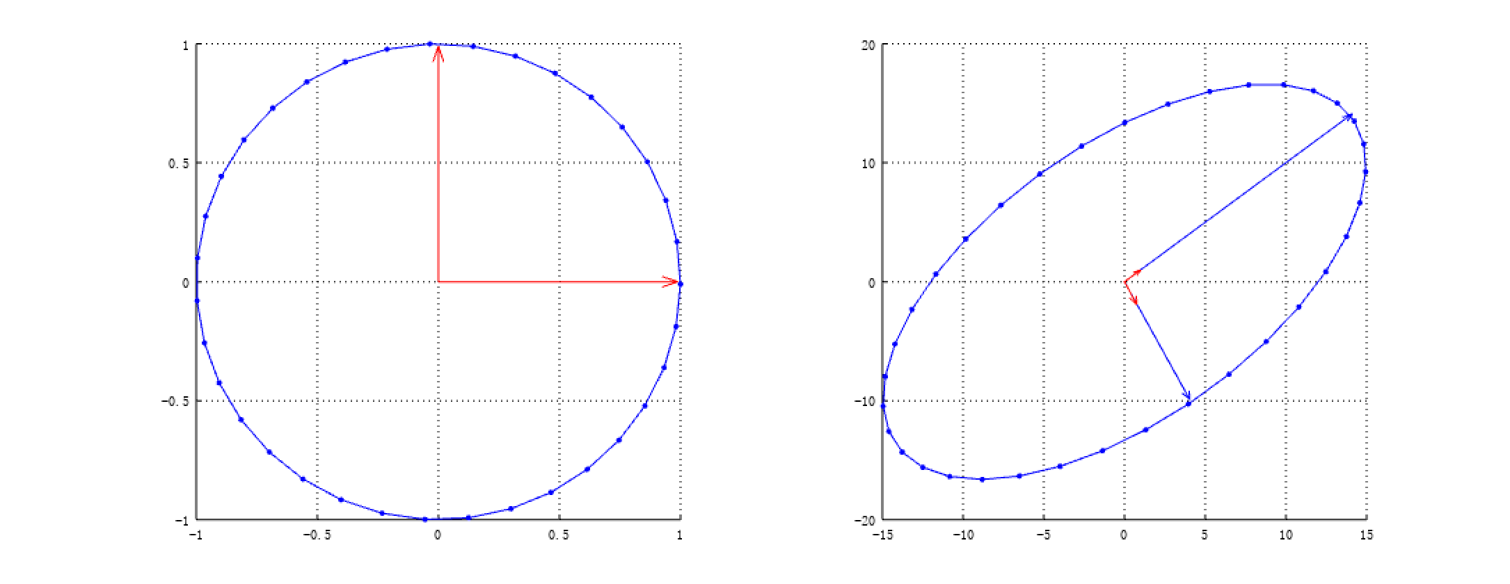$\begin{aligned} \vec{v_{1}} \vec{v_{2}} \vec{v_{3}}, . . . \vec{v_{n}} \to & \vec{u_{1}}, \vec{u_{2}}, \vec{u_{3}}, . . . \vec{u_{n}} \\ σ_{1}, σ_{2}, σ_{3}, . . . σ_{n} \end{aligned}$

Recall that we can transform $A$ at every direction, then generate another direction as new coordinate direction. So we have $A \vec{v_{1}} = σ_{1} \vec{u_{1}} A \vec{v_{2}} = σ_{2} \vec{u_{2}} ⋮ A \vec{v_{j}} = σ_{j} \vec{u_{j}}$

$\begin{aligned} (\begin{array}{c} A \end{array}) (\begin{array}{c} \vec{v_{1}}, \vec{v_{2}}, \dots, \vec{v_{n}} \end{array}) = (\begin{array}{c} \vec{u_{1}}, \vec{u_{2}}, \dots, \vec{u_{n}} \end{array}) (\begin{array}{c} σ_{1} & 0 & \dots & 0 \\ 0 & σ_{2} & \dots & 0 \\ ⋮ & ⋮ & ⋱ & ⋮ \\ 0 & 0 & \dots & σ_{n} \end{array}) \\ C^{m \times n} C^{n \times n} C^{m \times n} C^{n \times n} \end{aligned}$ Which is $A_{m \times n} V_{n \times n} = {\hat{U}}_{m \times n} {\hat{Σ}}_{n \times n}$

$\begin{aligned} A_{m \times n} V_{n \times n} & = {\hat{U}}_{m \times n} {\hat{Σ}}_{n \times n} \\ (A_{m \times n} V_{n \times n} V_{n \times n}^{- 1} & = {\hat{U}}_{m \times n} {\hat{Σ}}_{n \times n} V_{n \times n}^{- 1} \\ A_{m \times n} & = {\hat{U}}_{m \times n} {\hat{Σ}}_{n \times n} V_{n \times n}^{- 1} \\ = {\hat{U}}_{m \times n} {\hat{Σ}}_{n \times n} V_{n \times n}^{T} \end{aligned}$

We need do something to the equation in order to continue the deduction. First we stretch matrice $\hat{Σ}$ vertically to $m \times n$ size. Then stretch $\hat{U}$ horizonly to $m \times m$ , we can set any value to the right entries.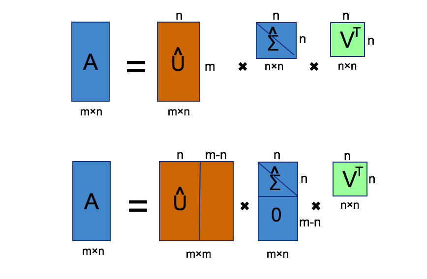

Due to the fact we need calculate $U^{- 1}$ and $V^{- 1}$ , the equation is adjusted to $A_{m \times n} = U_{m \times m} Σ_{m \times n} V_{n \times n}^{T}$ For furture convenience, we need sort all $σ s$ , which means: $σ_{1} \geq σ_{2} \geq σ_{3} \geq \dots \geq σ_{m}$ . #### How to calculate $U$ , $V^{T}$ and $Σ$ To Decompose matrice $A$ , we need calculate $U$ , $V^{T}$ and $Σ$ . Remember that $U^{T} = U^{- 1}$ and $V^{T} = V^{- 1}$ , we will use the property next.

$\begin{aligned} A & = U Σ V^{T} \end{aligned}$

$\begin{aligned} A A^{T} & = U Σ V^{T} (U Σ V^{T})^{T} \\ = U Σ V^{T} V Σ^{T} U^{T} \\ = U Σ V^{- 1} V Σ^{T} U^{T} \\ = U Σ I Σ^{T} U^{T} \\ = U Σ^{2} U^{T} \end{aligned}$

$\begin{aligned} (A A^{T}) U & = (U Σ^{2} U^{T}) U \\ = (U Σ^{2}) U^{- 1} U \\ = U Σ^{2} \end{aligned}$

$\begin{aligned} A^{T} A & = (U Σ V^{T})^{T} U Σ V^{T} \\ = V Σ^{T} U^{T} U Σ V^{T} \\ = V Σ^{T} U^{T} U Σ V^{T} \\ = V Σ^{T} U^{- 1} U Σ V^{T} \\ = V Σ^{T} I Σ V^{T} \\ = V Σ^{2} V^{T} \end{aligned}$

$\begin{aligned} (A^{T} A) V & = (V Σ^{2} V^{T}) V \\ = (V Σ^{2}) V^{- 1} V \\ = V Σ^{2} \end{aligned}$

Image Compression

Firstly, let's look at the process of compressing a picture, the left picture is original grayscale image. On the right, under different compress rate, we can see pictures after reproducing. Before compress, the size of the picture is 1775K byte. Then the picture is almost the same, when we compress which into 100K byte size, which means we can save 90% storage space

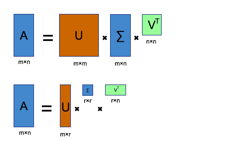
To compress a piture, you just decompose the matrice through SVD, then instead of using the original $U_{m \times m}$ , $Σ_{m \times n}$ and $U_{n \times n}$ , we shrink every matrice to new size $U_{m \times r}$ , $Σ_{r \times r}$ and $U_{r \times n}$ . The final $s i z e (R)$ is still $m \times n$ , but we abandon some entries since these entries are not so important than these we have reserved.

%% octave: core code of svd compressions
X = imread(filename);  
[U S V] = svd(double(X));
R = U(:,1:r)*S(1:r,1:r)*V(:,1:r)';

Summary

Today we have learned mathmatics backgroud on SVD, including linear transformation and EigenVector&EigenVaule. Before SVD, we first talked about EigenValue Decomposition. Finally, Singular Vaule Decomposition is very easy to be deduced. In the last section, we took an example see how SVD be applied to image compression field.

Now, it comes to the topic how to save our storage of a 32G iPhone7, the coclusion is obvious: using SVD compress image to shrink the size of our photos.

Reference

https://www.youtube.com/watch?v=EokL7E6o1AE
https://www.youtube.com/watch?v=cOUTpqlX-Xs
https://www.youtube.com/channel/UCYO_jab_esuFRV4b17AJtAw
https://yhatt.github.io/marp/
https://itunes.apple.com/cn/itunes-u/linear-algebra/id354869137
http://www.ams.org/samplings/feature-column/fcarc-svd
https://www.cnblogs.com/LeftNotEasy/archive/2011/01/19/svd-and-applications.html