Gaussian Discriminant Analysis

Preface

There are many classification algorithm such as Logistic Regression, SVM and Decision Tree etc. Today we'll talk about Gaussian Discriminant Analysis(GDA) Algorithm, which is not so popular. Actually, Logistic Regression performance better than GDA because it can fit any distributions from exponential family. However, we can learn more knowledge about gaussian distribution from the algorithm which is the most import distribution in statistics. Furthermore, if you want to understand Gaussian Mixture Model or Factor Analysis, GDA is a good start.

We, firstly, talk about Gaussian Distribution and Multivariate Gaussian Distribution, in which section, you'll see plots about Gaussian distributions with different parameters. Then we will learn GDA classification algorithm. We'll apply GDA to a dataset and see the consequnce of it.

Multivariate Gaussian Distribution

Gaussian Distribution

As we known that the pdf(Probability Distribution Function) of gaussian distribution is a bell-curve, which is decided by two parameters $\mu$ and ${\sigma }^2$. The figure below shows us a gaussian distribution with $\mu =0$ and ${\sigma }^2=1$, which is often referred to $\mathcal{N}(\mu ,{\sigma }^2)$. Thus, Figure1 is distributed normally with $\mathcal{N}(0,1)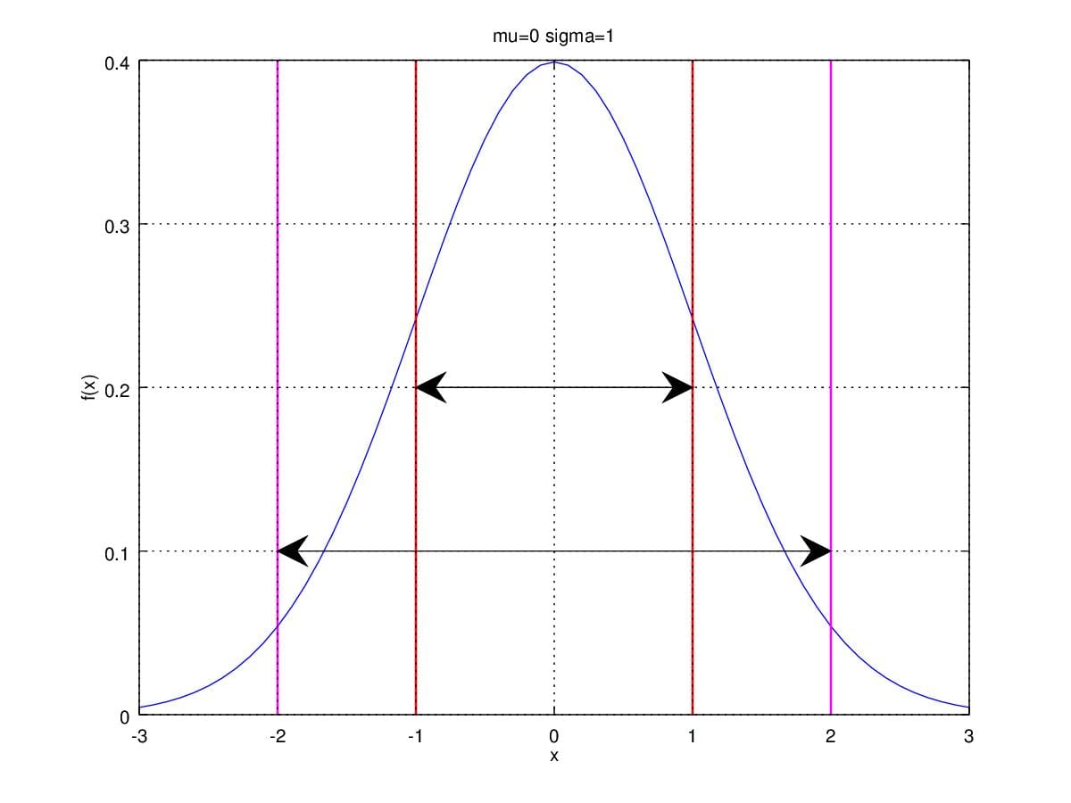$. Figure 1. Gaussian Distribution with $\mu =0$ and ${\sigma }^2=1$.

Actually, parameter $\mu$ and ${\sigma }^2$ are exactly the mean and the variance of the distribution. Therefore, $\sigma$ is the stand deviation of normal distribution. Let's take a look at area between red lines and magenta lines, which are respectively range from $\mu \pm \sigma$ and from $\mu \pm 2\sigma$. The area between redlines accounts for 68.3% of the total area under the curve. That is, there are 68.3% samples are between $\mu -\sigma$ and $\mu +\sigma$ . Likely, there are 95.4% samples are between $\mu -2\sigma$ and $\mu +2\sigma$.

You must want to know how these two parameter influence the shape of PDF of gaussian distribution. First of all, when we change $\mu$ with fixed ${\sigma }^2$, the curve is the same as before but move along the random variable axis.

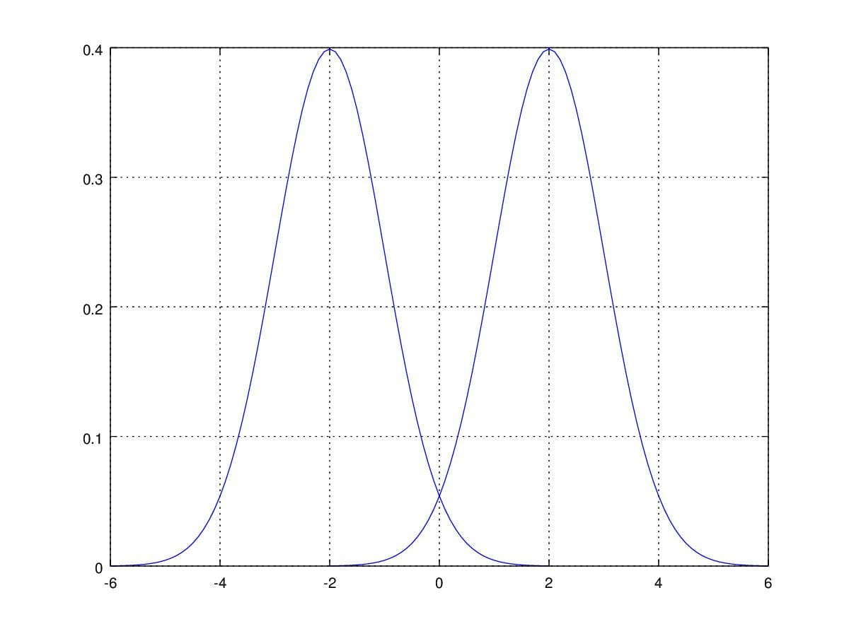
Figure 2. Probability Density Function curver with $\mu =\pm 2$ and $\sigma =1$.

So, what if when we change $\sigma$ then? Figure3. illustrates that smaller $\sigma$ lead to sharper shape of pdf. Conversely, larger $\sigma$ brings us broader curves.

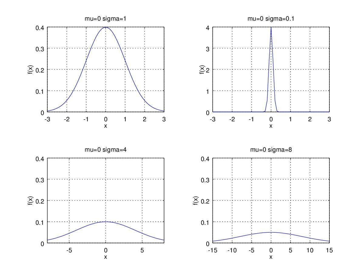
Figure 3. Probability Density Function curver with $\mu =0$ and change $\sigma$.

Some may wonder what is the form of $p(x)$ of a gaussian distribution, I just demonstrate here, you can compare Normal distribution with Multivariate Gaussian.

$$\mathcal{N}\mathcal{(}\mathcal{x}\mathcal{|}\mu \mathcal{,}{\sigma }^{\mathcal{2}}\mathcal{)}=\frac{1}{\sqrt{2\pi }\sigma }{e}^{-\frac{1}{2}\frac{(x-\mu {)}^2}{{\sigma }^2}}$$

Multivariate Gaussian

For convenience, we first see what is form of Multivariate Guassian Distribution:

$$\mathcal{N}\mathcal{(}\mathcal{x}\mathcal{|}\mu \mathcal{,}\mathcal{\Sigma }\mathcal{)}=\frac{1}{{(2\pi )}^{\frac{d}{2}}|\mathrm{\Sigma }{|}^{\frac{1}{2}}}{e}^{-\frac{1}{2}(x-\mu {)}^T{\mathrm{\Sigma }}^{-1}(x-\mu )}$$

where $\mu$ is the mean, $\mathrm{\Sigma }$ is the covariance matrices, $d$ is the dimension of random variable $x$, specfically, 2-dimensional gaussian distribution, we have:

$$\mathcal{N}\mathcal{(}\mathcal{x}\mathcal{|}\mu \mathcal{,}\mathcal{\Sigma }\mathcal{)}=\frac{1}{\sqrt{2\pi }|\mathrm{\Sigma }{|}^{\frac{1}{2}}}{e}^{-\frac{1}{2}(x-\mu {)}^T{\mathrm{\Sigma }}^{-1}(x-\mu )}$$

In order to get an intuition of Multivariate Guassian Distribution, We first take a look at a distribution with $\mu =\left(\begin{array}{c}0\\ 0\end{array}\right)$ and $\mathrm{\Sigma }=\left(\begin{array}{cc}1& 0\\ 0& 1\end{array}\right)$.

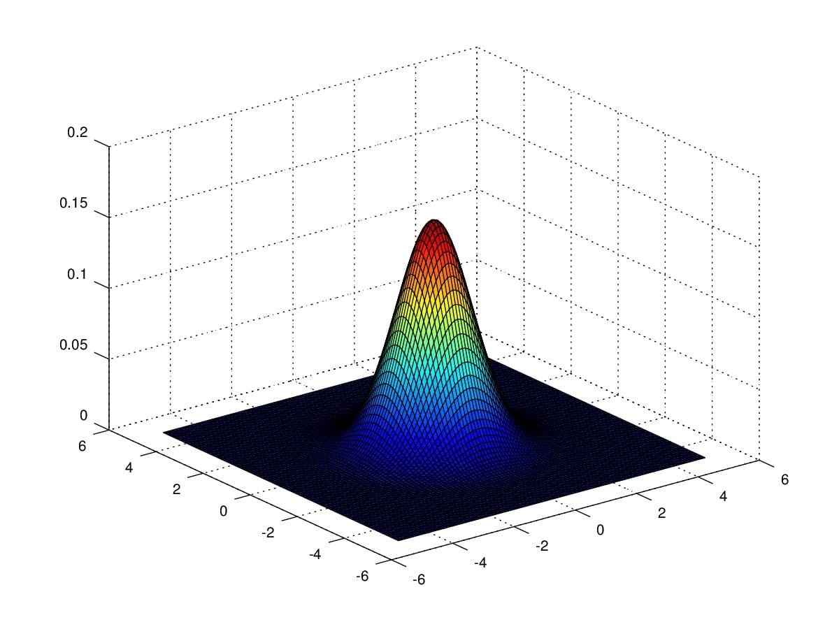
Figure 4. 2-dimensional gaussian distribution with $\mu =\left(\begin{array}{c}0\\ 0\end{array}\right)$ and $\mathrm{\Sigma }=\left(\begin{array}{cc}1& 0\\ 0& 1\end{array}\right)$.

Notice that the the figure is rather than a curve but a 3-dimensional diagram. Just like normal distribution pdf, $\sigma$ determines the shape of the figure. However, there are 4 entries of $\mathrm{\Sigma }$ can be changed in this example. Given that we need compute $|\mathrm{\Sigma }|$ as denominator and ${\mathrm{\Sigma }}^{-1}$ which demands non-zero determinant of $\mathrm{\Sigma }$, we must keep in mind that $|\mathrm{\Sigma }|$ is positive.

1. change $\mu$

Rather than change $\mathrm{\Sigma }$, we firstly take a look at how the contour looks like when changing $\mu$. Figure 5. illustrates the contour variation when changing $\mu$. As we can see, we only move the center of the contour during the variation of $\mu$. i.e. $\mu$ detemines the position of pdf rather than the shape. Next, we will see how entries in $\mathrm{\Sigma }$ influence the shape of pdf.

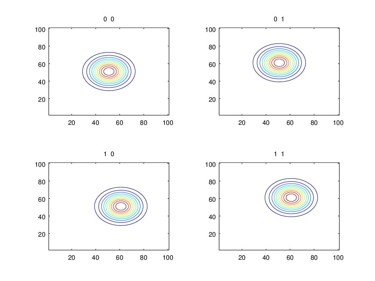
Figure 5. Contours when change $\mu$ with $\mathrm{\Sigma }=\left(\begin{array}{cc}1& 0\\ 0& 1\end{array}\right)$.

2. change diagonal entries of $\mathrm{\Sigma }$

If scaling diagonal entries, we can see from figure 6. samples are concentrated to a smaller range when change $\mathrm{\Sigma }$ from $\left(\begin{array}{cc}1& 0\\ 0& 1\end{array}\right)$ to $\left(\begin{array}{cc}0.3& 0\\ 0& 0.3\end{array}\right)$. Similarly, if we alter $\mathrm{\Sigma }$ to $\left(\begin{array}{cc}3& 0\\ 0& 3\end{array}\right)$, then figure will spread out.

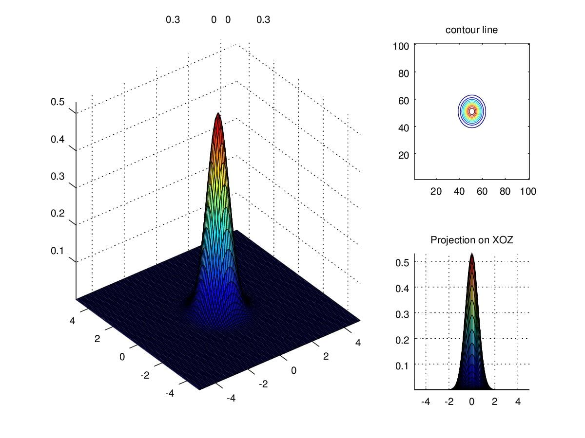
Figure 6. Density when scaling diagonal entries to 0.3.

What if we change only one entry of the diagonal? Figure 7. shows the variation of the density when change $\mathrm{\Sigma }$ to $\left(\begin{array}{cc}1& 0\\ 0& 5\end{array}\right)$. Notice the parameter spuashes and stretches the figure along coordinate axis.

Figure 7. Density when scaling one of the diagonal entries.

3. change secondary diagonal entries of $\mathrm{\Sigma }$

We now try to change entries along secondary diagonal. Figure 8. demonstrates that the variation of density is no longer parallel to $X$ and $Y$ axis, where $\mathrm{\Sigma }=\left(\begin{array}{cc}1& 0.5\\ 0.5& 1\end{array}\right)$.

Figure 8. Density when scaling secondary diagonal entries to 0.5

When we alter secondary entries to negative 0.5, the direction of contour presents a mirror to contour when positive.

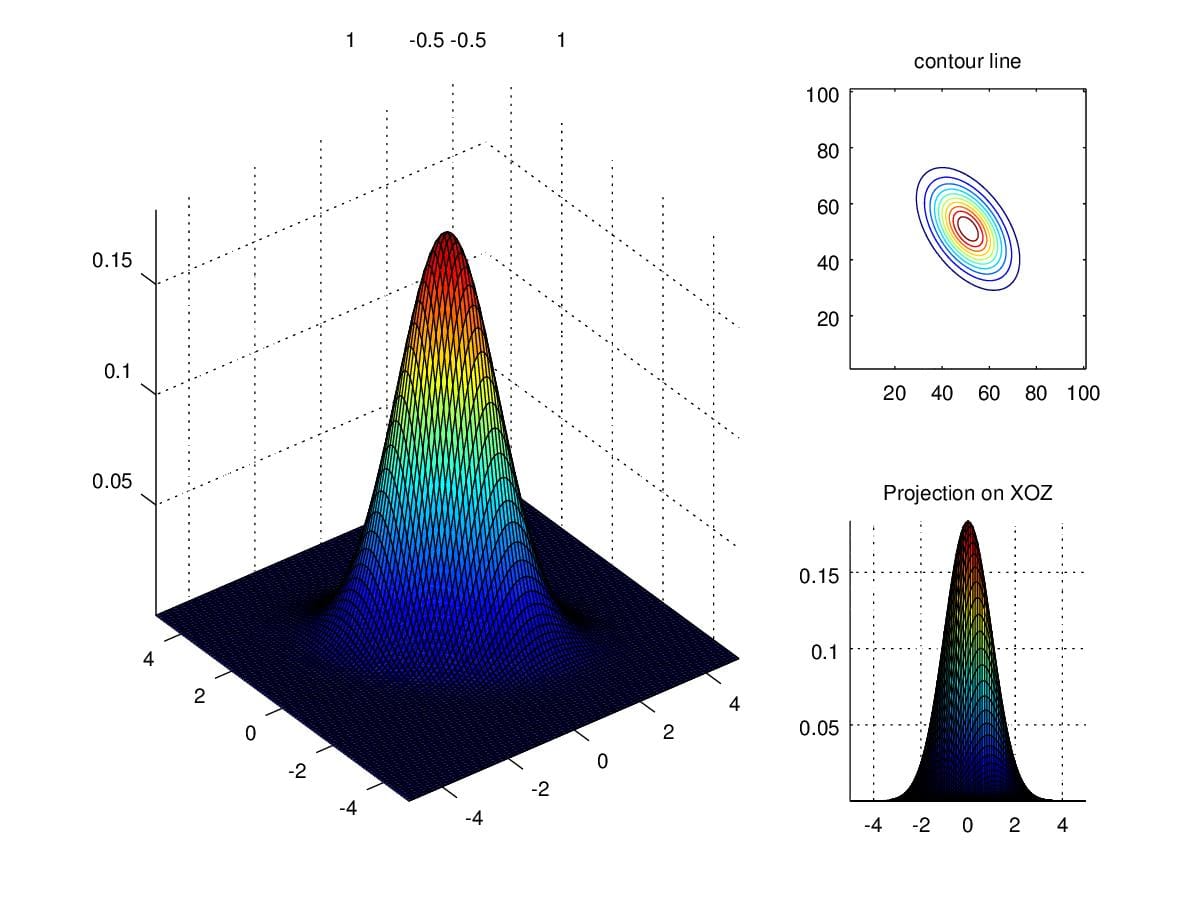
Figure 9. Density when scaling secondary diagonal entries to -0.5

In light of the importance of determinant of $\mathrm{\Sigma }$, what will happen if the determinant is close to zero. Actually, we can, informally, take determinant of a matrice as the volume of which. Similarly, when determinant is smaller, the volume under density curve become smaller. Figure 10. illustrates the circumstance we talked above where $\mathrm{\Sigma }=\left(\begin{array}{cc}1& 0.99\\ 0.99& 1\end{array}\right)$.

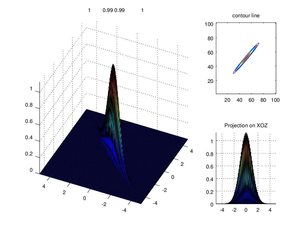
Figure 10. Density when determinant is close to zero.

Gaussian Discriminant Analysis

Intuition

When input features $x$ are continuous variables, we can use GDA classify data. Firstly, let's take a look at how GDA to do the job. Figure 11. show us two gaussian distributions, they share the same covariance $\mathrm{\Sigma }=\left(\begin{array}{cc}1& 0\\ 0& 1\end{array}\right)$ , and repectively with parameter ${\mu }_0=\left(\begin{array}{c}1\\ 1\end{array}\right)$ and ${\mu }_1=\left(\begin{array}{c}-1\\ -1\end{array}\right)$. Imagine you have some data which fall into the cover of the first and second Gaussian Distribution. If we can find such distributions to fit the data, then we'll have the capcity to decide which is new data coming from, the first or the second one.

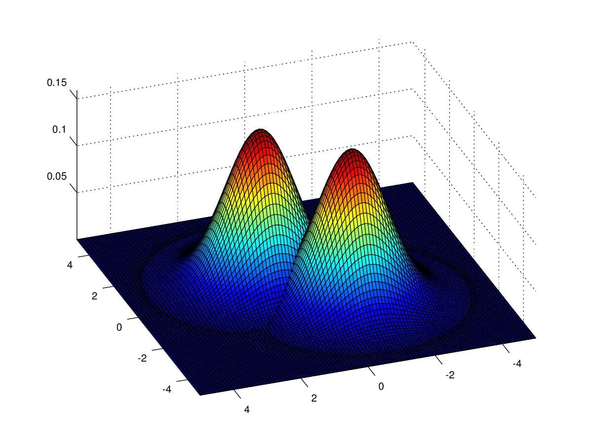
Figure 11. Two gaussian distributions with respect to ${\mu }_0=\left(\begin{array}{c}1\\ 1\end{array}\right)$ and ${\mu }_1=\left(\begin{array}{c}-1\\ -1\end{array}\right)$ , and $\mathrm{\Sigma }=\left(\begin{array}{cc}1& 0\\ 0& 1\end{array}\right)$

Specifically, let's look at a concrete example, Figure 12 are samples drawn from two Gaussian distribution. There are 100 blue '+'s and 100 red 'o's. Assume that we have such data to be classified. We can apply GDA to solve the problem.

CODE:

%% octave
pkg load statistics

m=200;
n=2;
rp=mvnrnd([1 1],[1 0;0 1],m/2);%生成正样本1
rn=mvnrnd([4 4],[1 0;0 1],m/2);%生成负样本0
y=[ones(m/2,1);zeros(m/2,1)];

figure;hold on;

plot3(rp(:,1),rp(:,2),y(1:m/2,1),'b+');
plot3(rn(:,1),rn(:,2),y(m/2+1:m,1),'ro');
axis([-3 8 -3 8]);

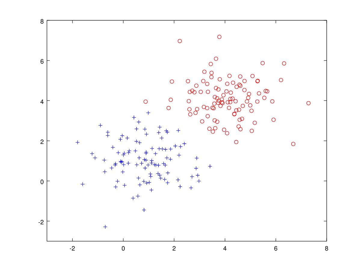
Figure 12. 200 samples drawn from two Gaussian Distribution with parameters ${\mu }_0=\left[\begin{array}{c}1\\ 1\end{array}\right],{\mu }_1=\left[\begin{array}{c}4\\ 4\end{array}\right],\mathrm{\Sigma }=\left[\begin{array}{cc}1& 0\\ 0& 1\end{array}\right]$.

Definition

Now, let's define the algorithm. Firstly we assume discrete random variable classes $y$ are distributed Bernoulli and parameterized by $\varphi$, then we have:

$$y\sim \mathrm{B}\mathrm{e}\mathrm{r}\mathrm{n}\mathrm{o}\mathrm{u}\mathrm{l}\mathrm{l}\mathrm{i}(\varphi )$$

Concretely, the probablity of $y=1$ is $\varphi$, and $1-\varphi$ when $y=0$. We can simplify two equations to one:

$p(y|\varphi )={\varphi }^y(1-\varphi {)}^{1-y}$

Apparently, $p(y=1|\varphi )=\varphi$ and $p(y=0|\varphi )=1-\varphi$ given that y can only be $0$ or $1$.

Another assumption is that we consider $x$ are subject to different Gaussian Distributions given different $y$. We assume the two Gaussian distributions share the same covariance and different $\mu$. Based on above all, then

$$p(x|y=0)=\frac{1}{(2\pi {)}^{\frac{d}{2}}|\mathrm{\Sigma }{|}^{\frac{1}{2}}}{e}^{-\frac{1}{2}(x-{\mu }_0{)}^T{\mathrm{\Sigma }}^{-1}(x-{\mu }_0)}$$

$$p(x|y=1)=\frac{1}{(2\pi {)}^{\frac{d}{2}}|\mathrm{\Sigma }{|}^{\frac{1}{2}}}{e}^{-\frac{1}{2}(x-{\mu }_1{)}^T{\mathrm{\Sigma }}^{-1}(x-{\mu }_1)}$$

i.e. $x|y=0\sim \mathcal{N}({\mu }_0,\mathrm{\Sigma })$ and $x|y=1\sim \mathcal{N}({\mu }_1,\mathrm{\Sigma })$. suppose we have $m$ samples, it is hard to compute $p(x^{(1)},x^{(2)},x^{(3)},\cdots ,x^{(m)}|y=0)$ or $p(x^{(1)},x^{(2)},x^{(3)},\cdots ,x^{(m)}|y=1)$ . In general, we assume the probabilty of $x^{(i)}$ $p(x^{(i)}|y=0)$ is independent to any $p(x^{(j)}|y=0)$, then we have:

$$p(X|y=0)=\prod _{i=1y^{(i)}\ne 1}^m\frac{1}{(2\pi {)}^{\frac{d}{2}}|\mathrm{\Sigma }{|}^{\frac{1}{2}}}{e}^{-\frac{1}{2}(x^{(i)}-{\mu }_0{)}^T{\mathrm{\Sigma }}^{-1}(x^{(i)}-{\mu }_0)}$$

Vice versa,

$$p(X|y=1)=\prod _{i=1y^{(i)}\ne 0}^m\frac{1}{(2\pi {)}^{\frac{d}{2}}|\mathrm{\Sigma }{|}^{\frac{1}{2}}}{e}^{-\frac{1}{2}(x^{(i)}-{\mu }_1{)}^T{\mathrm{\Sigma }}^{-1}(x^{(i)}-{\mu }_1)}$$

Here $X=(x^{(1)},x^{(2)},x^{(3)},\cdots ,x^{(m)})$. Now, we want to maximize $p(X|y=0)$ and $p(X|y=1)$. Why is that, because we hope find parameters that let $p(X|y=0)p(X|y=1)$ largest, based on that the samples are from the two Gaussian Distributions. These samples we have are more likely emerging. Thus, our task is to maximize $p(X|y=0)p(X|y=1)$ , we let

$$\mathcal{L}(\varphi ,{\mu }_0,{\mu }_1,\mathrm{\Sigma })=\arg maxp(X|y=0)p(X|y=1)=\arg max\prod _{i=1}^{m}p(x^{(i)},y^{(i)};\varphi ,{\mu }_0,{\mu }_1,\mathrm{\Sigma })$$

It's tough for us to maximize $\mathcal{L}(\varphi ,{\mu }_0,{\mu }_1,\mathrm{\Sigma })$. Notice function $\log$ is monotonic increasing. Thus, we can maximize $\log \mathcal{L}(\varphi ,{\mu }_0,{\mu }_1,\mathrm{\Sigma })$ instead of $\mathcal{L}(\varphi ,{\mu }_0,{\mu }_1,\varphi )$, then:

$$\begin{array}{rl}\ell (\varphi ,{\mu }_0,{\mu }_1,\mathrm{\Sigma })& =\log \mathcal{L}(\varphi ,{\mu }_0,{\mu }_1,\mathrm{\Sigma })\\ & =\arg max\log \prod _{i=1}^{m}p(x^{(i)},y^{(i)};\varphi ,{\mu }_0,{\mu }_1,\mathrm{\Sigma })\\ & =\arg max\log \prod _{i=1}^{m}p(x^{(i)}|y^{(i)};{\mu }_0,{\mu }_1,\mathrm{\Sigma })p(y^{(i)};\varphi )\\ & =\arg max\sum _{i=1}^{m}p(x^{(i)}|y^{(i)};{\mu }_0,{\mu }_1,\mathrm{\Sigma })+p(y^{(i)};\varphi )\\ & =\arg max\sum _{i=1}^{m}p(x^{(i)}|y^{(i)};{\mu }_0,{\mu }_1,\mathrm{\Sigma })+\sum _{i=1}^{m}p(y^{(i)};\varphi )\end{array}$$

By now, we have found a convex function with respect parameters ${\mu }_0,m{u}_1,\mathrm{\Sigma }$ and $\varphi$. Next section, we'll obtain these parameter through partial derivative.

Solution

To estimate these four parameters, we just apply partial derivative to $\ell$. Now we estimate $\varphi$ in the first place. We let $\frac{\partial \ell }{\partial \varphi }=0$, then

$$\begin{array}{rl}\frac{\partial \ell (\varphi ,{\mu }_0,{\mu }_1,\mathrm{\Sigma })}{\partial \varphi }=0& \Rightarrow \frac{\partial \arg max\sum _{i=1}^{m}p(x_i|y;{\mu }_0,{\mu }_1,\mathrm{\Sigma })+\sum _{i=1}^{m}p(y_i;\varphi )}{\partial \varphi }=0\\ & \Rightarrow \frac{\partial \sum _{i=1}^m\log p(y^{(i)};\varphi )}{\partial \varphi }=0\\ & \Rightarrow \frac{\partial \sum _{i=1}^m\log {\varphi }^{y^{(i)}}(1-\varphi {)}^{(1-y^{(i)})}}{\partial \varphi }=0\\ & \Rightarrow \frac{\partial \sum _{i=1}^m{y}^{(i)}\log \varphi +(1-y^{(i)})\log (1-\varphi )}{\partial \varphi }=0\\ & \Rightarrow \frac{\partial \sum _{i=1}^{m}1\{y^{(i)}=1\}\log \varphi +1\{y^{(i)}=0\}\log (1-\varphi )}{\partial \varphi }=0\\ & \Rightarrow \varphi =\frac{1}{m}\sum _{i=1}^{m}1\{y^{(i)}=1\}\end{array}$$

Note that ${\mu }_0$ and ${\mu }_1$ is symmetry in the equation, thus, we need only obtain one of them. Here we take the derivative to ${\mu }_0$

$$\begin{array}{rl}\frac{\partial \ell (\varphi ,{\mu }_0,{\mu }_1,\mathrm{\Sigma })}{\partial {\mu }_0}=0& \Rightarrow \frac{\partial \arg max\sum _{i=1}^{m}p(x_i|y;{\mu }_0,{\mu }_1,\mathrm{\Sigma })+\sum _{i=1}^{m}p(y_i;\varphi )}{\partial {\mu }_0}=0\\ & \Rightarrow \frac{\partial \sum _{i=1}^m\log p(x^{(i)}|y^{(i)};{\mu }_0,{\mu }_1,\mathrm{\Sigma })}{\partial {\mu }_0}=0\\ & \Rightarrow \frac{\partial \sum _{i=1}^m\log \frac{1}{(2\pi {)}^{\frac{d}{2}}|\mathrm{\Sigma }{|}^{\frac{1}{2}}}{e}^{-\frac{1}{2}(x^{(i)}-{\mu }_0{)}^T{\mathrm{\Sigma }}^{-1}(x^{(i)}-{\mu }_0)}}{\partial {\mu }_0}=0\\ & \Rightarrow 0+\frac{\partial \sum _{i=1}^m-\frac{1}{2}(x^{(i)}-{\mu }_0{)}^T{\mathrm{\Sigma }}^{-1}(x^{(i)}-{\mu }_0)}{\partial {\mu }_0}=0\end{array}$$

We have $\frac{\partial X^{T}AX}{\partial X}=(A+A^T)X$，let $(x^{(i)}-{\mu }_0)=X$, then,

$$\begin{array}{rl}\frac{\partial \ell (\varphi ,{\mu }_0,{\mu }_1,\mathrm{\Sigma })}{\partial {\mu }_0}=0& \Rightarrow 0+\frac{\partial \sum _{i=1}^m-\frac{1}{2}(x^{(i)}-{\mu }_0{)}^T{\mathrm{\Sigma }}^{-1}(x^{(i)}-{\mu }_0)}{\partial {\mu }_0}=0\\ & \Rightarrow \sum _{i=1}^m-\frac{1}{2}(({\mathrm{\Sigma }}^{-1}{)}^T+{\mathrm{\Sigma }}^{-1})(x^{(i)}-{\mu }_0)\cdot (-1)=0\\ & \Rightarrow \sum _{i=1}^{m}1\{y^{(i)}=0\}{x}^{(i)}=\sum _{i=1}^{m}1\{y^{(i)}=0\}{\mu }_0\\ & \Rightarrow {\mu }_0=\frac{\sum _{i=1}^{m}1\{y^{(i)}=0\}{x}^{(i)}}{\sum _{i=1}^{m}1\{y^{(i)}=0\}}\end{array}$$

Simlarly,

$${\mu }_1=\frac{\sum _{i=1}^{m}1\{y^{(i)}=1\}{x}^{(i)}}{\sum _{i=1}^{m}1\{y^{(i)}=1\}}$$

Before calculate $\mathrm{\Sigma }$, I first illustrate the truth that $\frac{\partial |\mathrm{\Sigma }|}{\partial \mathrm{\Sigma }}=|\mathrm{\Sigma }|{\mathrm{\Sigma }}^{-1},\frac{\partial {\mathrm{\Sigma }}^{-1}}{\partial \mathrm{\Sigma }}=-{\mathrm{\Sigma }}^{-2}$, then

$$\begin{array}{rl}\frac{\partial \ell (\varphi ,{\mu }_0,{\mu }_1,\mathrm{\Sigma })}{\partial \mathrm{\Sigma }}=0& \Rightarrow \frac{\partial \sum _{i=1}^m\log p(x^{(i)}|y^{(i)};{\mu }_0,{\mu }_1,\mathrm{\Sigma })+\sum _{i=1}^m\log p(y^{(i)};\varphi )}{\partial \mathrm{\Sigma }}=0\\ & \Rightarrow \frac{\partial \sum _{i=1}^m\log \frac{1}{(2\pi {)}^{\frac{d}{2}}|\mathrm{\Sigma }{|}^{\frac{1}{2}}}{e}^{-\frac{1}{2}(x^{(i)}-{\mu }_{y^{(i)}}{)}^T{\mathrm{\Sigma }}^{-1}(x^{(i)}-{\mu }_{y^{(i)}})}}{\partial \mathrm{\Sigma }}=0\\ & \Rightarrow \frac{\partial \sum _{i=1}^m-\frac{d}{2}\log 2\pi }{\partial \mathrm{\Sigma }}+\frac{\partial \sum _{i=1}^m-\frac{1}{2}\log |\mathrm{\Sigma }|}{\partial \mathrm{\Sigma }}+\frac{\partial \sum _{i=1}^m-\frac{1}{2}(x^{(i)}-{\mu }_{y^{(i)}}{)}^T{\mathrm{\Sigma }}^{-1}(x^{(i)}-{\mu }_{y^{(i)}})}{\partial \mathrm{\Sigma }}=0\\ & \Rightarrow \frac{\partial \sum _{i=1}^m-\frac{1}{2}\log |\mathrm{\Sigma }|}{\partial \mathrm{\Sigma }}+\frac{\partial \sum _{i=1}^m-\frac{1}{2}(x^{(i)}-{\mu }_{y^{(i)}}{)}^T{\mathrm{\Sigma }}^{-1}(x^{(i)}-{\mu }_{y^{(i)}})}{\partial \mathrm{\Sigma }}=0\\ & \Rightarrow m\frac{1}{|\mathrm{\Sigma }|}|\mathrm{\Sigma }|{\mathrm{\Sigma }}^{-1}+\sum _{i=1}^m(x^{(i)}-{\mu }_{y^{(i)}}{)}^T(x^{(i)}-{\mu }_{y^{(i)}})(-{\mathrm{\Sigma }}^{-2}))=0\\ & \Rightarrow \mathrm{\Sigma }=\frac{1}{m}\sum _{i=1}^m(x^{(i)}-{\mu }_{y^{(i)}})(x^{(i)}-{\mu }_{y^{(i)}}{)}^T\end{array}$$

In spite of the harshness of the deducing, the outcome are pretty beautiful. Next, we will apply these parameters and see how the estimation performance.

Apply GDA

Notice the data drawn from two Gaussian Distribution is random, thus, if you run the code, the outcome may be different. However, in most cases, distributions drawn by estimated parameters are roughly the same as the original distributions.

$$\begin{array}{rl}& \varphi =0.5\\ & {\mu }_0=\left[\begin{array}{c}4.0551\\ 4.1008\end{array}\right]\\ & {\mu }_1=\left[\begin{array}{c}0.85439\\ 1.03622\end{array}\right]\\ & \mathrm{\Sigma }=\left[\begin{array}{cc}1.118822& -0.058976\\ -0.058976& 1.023049\end{array}\right]\end{array}$$

From Figure 13, We can see contours of two Gaussian distribution, and most of samples are correctly classified.

CODE:

%% octave 
phi=length(find(y==1))/m;
mu_0 = sum(rn)/length(find(y==0))
mu_1 = sum(rp)/length(find(y==1))
X = [rp;rn];
X_mu1 = X(find(y==1),:)-mu_1;
X_mu0 = X(find(y==0),:)-mu_0;
X_mu = [X_mu1; X_mu1];
sigma = (X_mu'*X_mu)/m

[x1 y1]=meshgrid(linspace(-3,8,100)',linspace(-3,8,100)');
X1=[x1(:) y1(:)];
z1=mvnpdf(X1,mu_1,sigma);
contour(x1,y1,reshape(z1,100,100),8);
hold on;
z2=mvnpdf(X1,mu_0,sigma);
contour(x1,y1,reshape(z2,100,100),8);

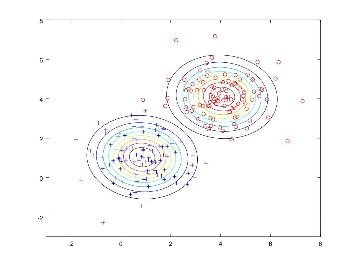
Figure 13. Contours drawn from parameters estimated.

In fact, we can compute the probability of each data point to predict which distribution it is more likely belongs, for example, if we want to predict $x=\left(\begin{array}{c}0.88007\\ 3.9501\end{array}\right)$ is more of the left distribution or the right, we apply $x$ to these two distribution:

$$\begin{array}{rl}p(x=\left[\begin{array}{c}0.88\\ 3.95\end{array}\right]|y=0)=& \frac{1}{2\pi |\mathrm{\Sigma }{|}^{\frac{1}{2}}}{e}^{-\frac{1}{2}{\left[\begin{array}{c}{x}_1-{\mu }_1\\ x_2-{\mu }_2\end{array}\right]}^T{\mathrm{\Sigma }}^{-1}\left[\begin{array}{c}{x}_1-{\mu }_1\\ x_2-{\mu }_2\end{array}\right]}\\ =& \frac{1}{2\pi {\left|\begin{array}{cc}1.1188& -0.059\\ -0.059& 1.023\end{array}\right|}^{\frac{1}{2}}}{e}^{-\frac{1}{2}{\left[\begin{array}{c}-3.175\\ -0.151\end{array}\right]}^T\left[\begin{array}{cc}0.896& -0.052\\ -0.0520& 0.98\end{array}\right]\left[\begin{array}{c}-3.175\\ -0.151\end{array}\right]}\\ =& \frac{1}{2\pi \sqrt{(1.141)}}{e}^{-\frac{1}{2}\times 9.11}=0.149\times 0.01=0.0015\end{array}$$

and

$$\begin{array}{rl}p(x=\left[\begin{array}{c}0.88\\ 3.95\end{array}\right]|y=1)& \frac{1}{2\pi |\mathrm{\Sigma }{|}^{\frac{1}{2}}}{e}^{-\frac{1}{2}{\left[\begin{array}{c}{x}_1-{\mu }_1\\ x_2-{\mu }_2\end{array}\right]}^T{\mathrm{\Sigma }}^{-1}\left[\begin{array}{c}{x}_1-{\mu }_1\\ x_2-{\mu }_2\end{array}\right]}\\ =& \frac{1}{2\pi {\left|\begin{array}{cc}1.1188& -0.059\\ -0.059& 1.023\end{array}\right|}^{\frac{1}{2}}}{e}^{-\frac{1}{2}{\left[\begin{array}{c}0.03\\ 2.91\end{array}\right]}^T\left[\begin{array}{cc}0.896& -0.052\\ -0.0520& 0.98\end{array}\right]\left[\begin{array}{c}0.03\\ 2.91\end{array}\right]}\\ =& \frac{1}{2\pi \sqrt{(1.141)}}{e}^{-\frac{1}{2}\times 8.336}=0.149\times 0.015=0.0022\end{array}$$

In light of the equivalency of $p(y=1)$ and $p(y=0)$ (both are $0.5$), we just compare$p(x=\left[\begin{array}{c}0.88\\ 3.95\end{array}\right]|y=1)$ to $p(x=\left[\begin{array}{c}0.88\\ 3.95\end{array}\right]|y=0)$. Apparently, this data point is predicted from the left distribution, which is a wrong assertion. Actually, in this example, we have only this data pointed classified incorrectly.

You may wonder why there is a blue line. It turns out that all the data point below the blue line will be considered as blue class. Otherwise, data points above the line is classified as the red class. How it work?

The blue line is decision boundary, if we know the expression of this line, the decision will be made easier. In fact GDA is a linear classifier, we will prove it later. Still, we see the data point above, if we just divide one probability to another, we just need find if the ratio larger or less than 1. For our example, the ratio is roughly 0.68, so the data point is classified to be the blue class.

$$\frac{p(x=\left[\begin{array}{c}0.88\\ 3.95\end{array}\right]|y=0)p(y=0)}{p(x=\left[\begin{array}{c}0.88\\ 3.95\end{array}\right]|y=1)p(y=1)}=\frac{0.0015}{0.0022}=0.68182<1$$

Figure 14. Decision Boundary

If we can obtain the expression of the ratio, that should be good. So given a new $x$, we predict problem is tranformed as followed:

$$x\in \text{redclass}\propto \mathcal{R}=\frac{p(x|y=1)p(y=1)}{p(x|y=0)p(y=0)}>1$$

which is equal to

$$\mathcal{R}=\log \frac{p(x|y=1)p(y=1)}{p(x|y=0)p(y=0)}=\log \frac{\varphi }{1-\varphi }+\log \frac{\mathcal{N}(x;{\mu }_1,\mathrm{\Sigma })}{\mathcal{N}(x;{\mu }_0,\mathrm{\Sigma })}>0$$

Then,

$$\begin{array}{rl}\mathcal{R}& =\log \frac{\frac{1}{(2\pi {)}^{\frac{d}{2}}|\mathrm{\Sigma }{|}^{\frac{1}{2}}}\exp (-\frac{1}{2}(x-{\mu }_1{)}^T{\mathrm{\Sigma }}^{-1}(x-{\mu }_1))}{\frac{1}{(2\pi {)}^{\frac{d}{2}}|\mathrm{\Sigma }{|}^{\frac{1}{2}}}\exp (-\frac{1}{2}(x-{\mu }_0{)}^T{\mathrm{\Sigma }}^{-1}(x-{\mu }_0))}+\log \frac{\varphi }{1-\varphi }\\ & =-\frac{1}{2}(x-{\mu }_1{)}^T{\mathrm{\Sigma }}^{-1}(x-{\mu }_1))+\frac{1}{2}(x-{\mu }_0{)}^T{\mathrm{\Sigma }}^{-1}(x-{\mu }_0))+\log \frac{\varphi }{1-\varphi }\\ & =-\frac{1}{2}{x}^T{\mathrm{\Sigma }}^{-1}x+{\mu }_1^T{\mathrm{\Sigma }}^{-1}x-\frac{1}{2}{\mu }_1^T{\mathrm{\Sigma }}^{-1}{\mu }_1+-\frac{1}{2}{x}^T{\mathrm{\Sigma }}^{-1}x-{\mu }_0^T{\mathrm{\Sigma }}^{-1}x+\frac{1}{2}{\mu }_0^T{\mathrm{\Sigma }}^{-1}{\mu }_0+\log \frac{\varphi }{1-\varphi }\\ & =({\mu }_0-{\mu }_1{)}^T{\mathrm{\Sigma }}^{-1}x-\frac{1}{2}{\mu }_1^T{\mathrm{\Sigma }}^{-1}{\mu }_1+\frac{1}{2}{\mu }_0^T{\mathrm{\Sigma }}^{-1}{\mu }_0+\log \frac{\varphi }{1-\varphi }\end{array}$$

Here, ${\mu }_1^T{\mathrm{\Sigma }}^{-1}x=x^T{\mathrm{\Sigma }}^{-1}{\mu }_1$ because it is a real number. For a real number $a=a^T$, moreover, ${\mathrm{\Sigma }}^{-1}$ is symmetric, so ${\mathrm{\Sigma }}^{-T}={\mathrm{\Sigma }}^{-1}$. Let's set $w^T=({\mu }_1-{\mu }_0{)}^T{\mathrm{\Sigma }}^{-1}$ and $w_0=-\frac{1}{2}{\mu }_1^T{\mathrm{\Sigma }}^{-1}{\mu }_1+\frac{1}{2}{\mu }_0^T{\mathrm{\Sigma }}^{-1}{\mu }_0+\log \frac{\varphi }{1-\varphi }$, then we have:

$$\mathcal{R}=\log \frac{p(x|y=1)p(y=1)}{p(x|y=0)p(y=0)}=w^{T}x+w_0$$

If you plug parameters in the formula, you will find:

$\mathcal{R}=-3.0279x_1-3.1701x_2+15.575=0$

It is the decision boundary(Figure 14.). Since you have got the decision boundary formula, it is convenient to use the decision boundary function predict if a data point $x$ belongs to the blue or red class. If $\mathcal{R}>0$, $x\in \text{red class}$, otherwise, $x\in \text{blue class}$.

Conclusion

Today, we have talked about Guassian Distribution and its Multivariate form. Then, we assume two groups of data drawn from Gaussian Distributions. We apply Gaussian Discriminant Analysis to the data. There are 200 data point, only one is misclassified. In fact we can deduce GDA to Logistic regression Algorithm(LR). But LR can not deduce GDA, i.e. LR is a better classifier, especially when we do not know the distribution of the data. However, if you have known that data is drawn from Gaussian Distribution, GDA is the better choice.

Reference

1. Andrew Ng http://cs229.stanford.edu/notes/cs229-notes2.pdf
2. https://en.wikipedia.org/wiki/Normal_distribution
3. https://en.wikipedia.org/wiki/Multivariate_normal_distribution
4. http://www.cnblogs.com/emituofo/archive/2011/12/02/2272584.html
5. http://m.blog.csdn.net/article/details?id=52190572
6. 张贤达《矩阵分析与应用》:156-158
7. http://www.tk4479.net/hujingshuang/article/details/46357543
8. http://www.chinacloud.cn/show.aspx?id=24927&cid=22
9. http://www.cnblogs.com/jcchen1987/p/4424436.html
10. http://www.xlgps.com/article/139591.html
11. http://www.matlabsky.com/thread-10308-1-1.html
12. http://classes.engr.oregonstate.edu/eecs/fall2015/cs534/notes/GaussianDiscriminantAnalysis.pdf