Spectral analysis (2)
Diffussion map
Eigenvalue decomposition of weighted graph laplacian is used to obtain diffusion map. The asymmetric matrix or transition matrix \(P=D^{-1}W\). The decomposition is: \[\begin{equation} P = D^{-1/2}S\Lambda S^\top D^{1/2} \end{equation}\] In fact, the random walk on the graph would give rise to the transition graph such that: \[\begin{equation} p^{t+1}= p^t D^{-1}W = p^t P \end{equation}\] where \(p\) is a initial state of the graph (vertices weight). That is, after a certain step of random walk on the graph, we would reach a steady state when any more random walk would not change the weight. Let \(Q=D^{-1/2}S\), then \(Q^{-1}=S^{\top} D^{1/2}\), we can derive \(P = Q\Lambda Q^{-1}\). The random walk above mentioned can then be represent: \[\begin{equation} \begin{aligned} P^t &= Q\Lambda Q^{-1}Q\Lambda Q^{-1}\cdots Q\Lambda Q^{-1} &= Q\Lambda^t Q \end{aligned} \end{equation}\] Since \(\Lambda\) is diagnoal, the random walk on a graph can be easily cacluted by using the eigenvalue decomposition outcome. The column of \(Q\) is the diffusion map dimensions.
Diffusion map example
To understand diffusion map, we here introduce an example data and run diffusion map on it. The data is a single cell fibroblasts to neuron data with 392 cells. We first download the data from NCBI and loaded the data to memory:
1 | import requests |
From the code as we can see that, we extract the cell types from the
data and stores it into the variable group. The rest part
of the data is the normalized gene expression count matrix.
To do the pre-processing, we first get the log-normalized count
matrix \(X\) and revert it to the
counts and apply log geomatric scaling to the count matrix as the
pre-processing then store it to matrix \(Y\). 1
2
3X = np.array(data.iloc[:, 5:]).T
X = np.power(2, X[np.apply_along_axis(np.var, 1, X)>0, :]) - 1
Y = np.log(gscale(X+0.5)).T1
2
3
4
5
6
7
8
9def gscale(X:np.ndarray) -> np.ndarray:
assert(X.all()>=0)
div_ = np.divide(X.T, np.apply_along_axis(lambda x:np.exp(np.mean(np.log(x))), 1,
X)).T
scale_ = np.apply_along_axis(np.median,0, div_)
sc = StandardScaler(with_mean=False)
sc.fit(X)
sc.scale_ = scale_
return sc.transform(X)
1 | pc = run_pca(Y, 100) |
We first take a look at the PCA figure which shows the first 2 PCs of
the dataset. PCA is a linear methods which cannot reflect cell fate
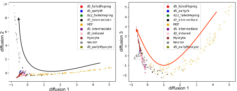
differentation process. 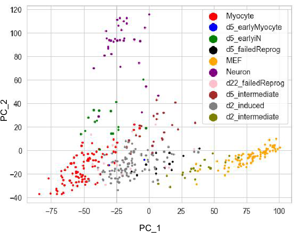 Since the diffusion map applied the Gaussian kernal during the distances
calculation, it usually a better way to capture the cell differentation
events. Here we show diffusion dimension 1,2 and 1,3. It's clear that
1,2 captures the cell differentation from fibroblasts to neuron, and 1,3
captures the differentiation from firoblasts to myocytes.
We can change the bandwidth from 7 to 100, which use the 100th
neareast neighbor as bandwidth instead of 7th. The following shows the
diffusion map that bandwidth=100. 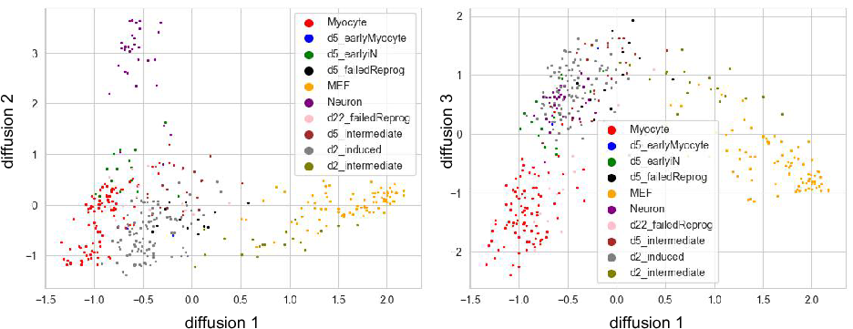
pseudo time by random walk
The eigenvalue decomposition of graph laplacian can also be used to
infer the pseudo time simulating the pseudo time of cell differentation
events. We here set top \(m\) cells
\(1/m\) of the progenitor cells (MEF)
and set other cell 0 as the initial state. Next, we perform random walk
to get new pesudotime \(u\) such that:
\[\begin{equation}
u = [\frac{1}{m}, \frac{1}{m}, \cdots, 0, \cdots 0](D^{-1}W)^t
\end{equation}\] By testing different number of random walk steps
we can check the new pseudo time \(u\).
Here we show time step equals to 1, 10, 100 and 200. From the figure we
can notice that after certain step, the pseudo time will not change
anymore. That means the random walk reaches the steady state. 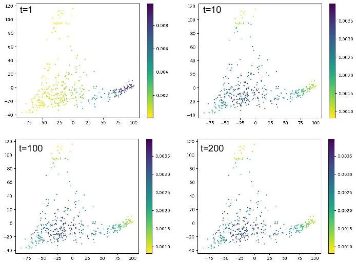
To test when can we reach the steady state, I use the graph we
mentioned in my last post Spectral
analysis (1):
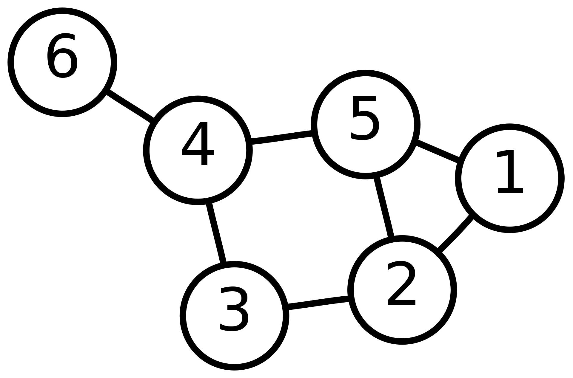
Here we random generate two initial states (\(v_1\), \(v_2\)) to do the random walk such that: \[\begin{equation} \begin{aligned} v_1 &= [0.15,0.41,0.54,0.9,0.62,0.93,0.1,0.46,0.01,0.88]\\ v_2 &= [0.89,0.93,0.07,0.41,0.52,0.88,0.43,0.09,0.1,0.2] \end{aligned} \end{equation}\]
From the the figure below we can see that \(v_1\) reaches the steady state in 30 steps
whereas \(v_2\) reaches steady state in
100 steps. In total, all these two initial state will reach the steady
state that would not change any longer. 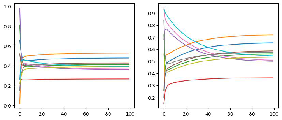
spectral clustering
The eigenvectors of graph Laplacian can also be used to do the
clustering. From the figure we can find clear cut using the 1st, 2nd and
the 3rd diffusion dimensions. In practice, we can use kmeans, DBSCAN,
leiden, louvain algorithm to perform clustering using the diffusion
dimensions. 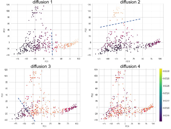
Appendix
PCA function
1 | def run_pca(mtx, n_components=2, random_state=2022): |
Affinity matrix function
1 | def affinity(R, k=7, sigma=None, log=False): |
Diffusion map function
1 | def diffusionMaps(R,k=7,sigma=None): |