Graph laplacian is familiar to computation science researcher, with
which we can perform spectral analysis such as diffusion map, eigenmap
or spectral clustering. Here, we discuss how to generalize the graph
laplacian to it's high-order form, i.e., Hodge laplacian.
Graph laplacian
In the previous post we know that the graph laplacian can be obtianed
by degree matrix \(D\) and adjacency
matrix \(A\) such that: \[\begin{equation}
L_0 = D - A
\end{equation}\]
We can find the adjacency matrix and degree matrix of the graph blow
with nine vertices:
However, there's anoth way to represent the graph laplacian. Before
that, we first introduce the incidence matrix of a graph. First, we can
convert an undirected graph to be directed just assign the direction of
edges by book keeping order. Next, let's construct the incidence matrix,
each row represent a vertex, and each colum is an edge. We set the entry
to be 1 if the the edge enter the vertex -1 when leave the vertex. Set 0
if there's no connection between a vertex and an edge. Thus the
incidence matrix of a graph \(G\) is
\(B\) such that: \[\begin{equation}
B_1 =
\begin{array}[r]{c | c c c c c c c}
& \cdots & [4,5] & [4,6]& [5,6]&
[6,7]& \cdots\\
\hline
\vdots & \cdots & & \cdots & &
\cdots & \\
4 & \cdots & -1 & -1 & 0 & 0
& \cdots\\
5 & \cdots & 1 & 0 & -1 & 0 &
\cdots\\
6 & \cdots & 0 & 1 & 1 & -1 &
\cdots\\
7 & \cdots & 0 & 0 & 0 & 1 &
\cdots\\
\vdots & \cdots & & \cdots & &
\cdots & \\
\end{array}
\end{equation}\] Next, let construct graph laplacian matrix using
\(B_1\). Actually, the graph laplacian
is: \[\begin{equation}
L_0=B_1 B_1^\top = \begin{array}[r]{c |c c c c c c c c c }
& 1 & 2 & 3 & 4 & 5 & 6 & 7 &
8 & 9\\
\hline
1& 1 & -1 & 0 & 0 & 0 & 0 & 0
& 0 & 0\\
2& -1 & 2 & -1 & 0 & 0 & 0 & 0
& 0 & 0\\
3& 0 & -1 & 1 & 0 & 0 & 0 & 0
& 0 & 0\\
4& 0 & 0 & 0 & 2 & -1 & -1 & 0
& 0 & 0\\
5& 0 & 0 & 0 & -1 & 2 & -1 & 0
& 0 & 0\\
6& 0 & 0 & 0 & -1 & -1 & 3 & -1
& 0 & 0\\
7& 0 & 0 & 0 & 0 & 0 & -1 & 1
& 0 & 0\\
8& 0 & 0 & 0 & 0 & 0 & 0 & 0
& 1 & -1\\
9& 0 & 0 & 0 & 0 & 0 & 0 & 0
& -1 & 1\\
\end{array}
\end{equation}\] As we can see that, \(L_0\) is the same as the that obtained from
degree matrix and adjacency matrix.
Zero eigenvaules of graph
laplacian
We know that for the application of diffusion map or spectral
analysis, we have to drop the first eigenvector due to its same values
and the eigenvaule is 0. The second eigenvector is also called fidler
vector. However, these applications usually created a connected graph.
Since the graph we show here is an unconnected graph. We can stop here
to take a guess: Is the zero eigenvaule still there, or if so, how many
zero eigenvaules?
Interestingly, the top 3 eigenvalues are all zero and we also have 3
connected components in the graph. Is this a coincidence or a property
of graph laplacian decomposition?
Furthermore, the top 3 eigenvectors corresponding to the zero
eigenvaules are also interesting. Notice that the first eigenvector can
differentiate the components \(\{4,5,6,7\}\) from the rest vectices.
Likewise, the second eigenvector select the connected component \(\{8,9\}\) and the third choose the
component \(\{1,2,3\}\).
In fact, in the field of Topological Data Analysis (TDA), the \(L_0\) is the special case of hodge
laplacian (\(L_k\)). The number of
connected components is call 0-dimensional cycles. And the graph
laplaican can capture these cycles. The 1-dimensional cycles are
correspond to holes, we will go into detail in the next section.
Hodge laplacian
We can see the graph laplacian zero-order of hodge laplacian, and the
formalu can be represented as: \[\begin{equation}
L_0 = \mathbf{0}^\top \mathbf{0} + B_1 B_1^\top
\end{equation}\]
You must ask where is \(B_2\) coming
from? We know that \(B_1\) captures the
relationship between vertices and edges. Thus, \(B_2\) captures the relationship between
edges and triangles. We can also define \(B_3\) to capture relationship between
triangles and tetrahedron and so on and so forth. So what is a triangle
or a tetrahedron in a graph? We would not go into the detail of the
thory of Simplex and Simplicial complex. Here we just need to know that
three connected vertices forms a triangle. Similarly, four connected
vertices forms a tetrahedron which is a high-order of triangles. To
define \(B_2\), of a graph \(G\), we would check the direction of an
edge \(e_j\) to the triangle \(\bigtriangleup_q\) it beblongs, if it has
the same direction as the triangle, the entry would be \(1\), if the direction is opposite, the
entry would be -1, otherwise the entry would be zero. Specifically:
With the definition, we can obtian \(B_2\) of the graph aforementioned: \[\begin{equation}
B_2 =
\begin{array}[r]{c | c }
& [4,5,6]\\
\hline
\vdots & \cdots \\
[4,5] & 1\\
[4,6] & -1\\
[5,6]& 1\\
[6,7] & 0\\
\vdots & \cdots \\
\end{array}
\end{equation}\]
We next introduce the normalized form and the decomposition of hodge
1-laplacian. The normalized form of hodge 1-laplacian is given:
\[\begin{equation}
\mathcal{L}_1 = {D}_2 {B}_1^\top {D}_1^{-1} {B}_1 + {B}_2 {D}_3
{B}_2^\top {D}_2^{-1}
\end{equation}\] where \(\mathbf{D}_1\) is the vertices degree
matrix, \({D}_2\) is \(\max{(\text{diag}(|{B}_2| \mathbf{1}),
\mathbf{I})}\) and \({D}_3\) is
\(\frac{1}{3}\mathbf{I}\). Since the
normalized \(L_1\) is not neccessarily
symmetric, we next need to define the symmetric normalized Hodge
1-Laplacian such that: \[\begin{equation}
\begin{aligned}
\mathcal{L}_1^s
& = {D}_2^{-1/2} \mathcal{L}_1 {D}_2^{1/2}\\
& = {D}_2^{1/2} {B}_1^\top {D}_1^{-1} {B}_1 {D}_2^{1/2} +
{D}^{-1/2} {B}_2 {D}_3 {B}_2^\top {D}_2^{-1/2}
\end{aligned}
\end{equation}\]
We use the graph with three holes to present hodge 1-laplacian:
We next can perform eigenvalues decomposition on \(\mathcal{L}_1\): \[\begin{equation}
\begin{aligned}
\mathcal{L}_1
& = \mathbf{D}_2^{1/2} \mathcal{L}_1^s
\mathbf{D}_2^{-1/2} \\
& = \mathbf{D}_2^{1/2} Q \Lambda Q^\top
\mathbf{D}_2^{-1/2} \\
& = \mathbf{U} \Lambda \mathbf{U}^{-1}
\end{aligned}
\end{equation}\] Interestingly, the top 3 eigenvector also all
zero which corresponding to the 3 holes, namely, the three 1-dimensional
cycles.
When it comes to the eigenvectors, we can also notice that the top
three eigenvectors are around the three holes.
In algebraic geometry, these the eigenvectors with zero eigenvaules
are called harmonic function or harmonic. These harmonic function around
holes is useful for some analysis like clustering to find the
1-dimensional cycles etc.
Conclusion
Today, we review the graph laplacian, and we can find the zeor
eigenvalues and theirs corresponding eigenvectors can be used to find
connected components. The high order graph laplacian hodge laplacian
have the similar properties, we presented the hodge 1-laplaican and its
eigenvalues decomposition. We can find that the zero eigenvalues
indicates the number of holes of a graph. Furthermore, the corresponding
eigenvectors with zero eigenvalues are around holes.
Eigenvalue decomposition of weighted graph laplacian is used to
obtain diffusion map. The asymmetric matrix or transition matrix \(P=D^{-1}W\). The decomposition is: \[\begin{equation}
P = D^{-1/2}S\Lambda S^\top D^{1/2}
\end{equation}\] In fact, the random walk on the graph would give
rise to the transition graph such that: \[\begin{equation}
p^{t+1}= p^t D^{-1}W = p^t P
\end{equation}\] where \(p\) is
a initial state of the graph (vertices weight). That is, after a certain
step of random walk on the graph, we would reach a steady state when any
more random walk would not change the weight. Let \(Q=D^{-1/2}S\), then \(Q^{-1}=S^{\top} D^{1/2}\), we can derive
\(P = Q\Lambda Q^{-1}\). The random
walk above mentioned can then be represent: \[\begin{equation}
\begin{aligned}
P^t &= Q\Lambda Q^{-1}Q\Lambda Q^{-1}\cdots Q\Lambda Q^{-1}
&= Q\Lambda^t Q
\end{aligned}
\end{equation}\] Since \(\Lambda\) is diagnoal, the random walk on a
graph can be easily cacluted by using the eigenvalue decomposition
outcome. The column of \(Q\) is the
diffusion map dimensions.
Diffusion map example
To understand diffusion map, we here introduce an example data and
run diffusion map on it. The data is a single cell fibroblasts to neuron
data with 392 cells. We first download the data from NCBI and loaded the
data to memory:
1
2
3
4
5
6
7
import requests url ='https://www.ncbi.nlm.nih.gov/geo/download/?acc=GSE67310&format=file&file=GSE67310%5FiN%5Fdata%5Flog2FPKM%5Fannotated.txt.gz' r = requests.get(url, allow_redirects=True) open('GSE67310.txt.gz','wb').write(r.content) data = pd.read_csv('GSE67310.txt.gz', sep='\t', index_col=0) data = data.loc[data['assignment']!='Fibroblast'] group = data['assignment']
From the code as we can see that, we extract the cell types from the
data and stores it into the variable group. The rest part
of the data is the normalized gene expression count matrix.
To do the pre-processing, we first get the log-normalized count
matrix \(X\) and revert it to the
counts and apply log geomatric scaling to the count matrix as the
pre-processing then store it to matrix \(Y\).
1
2
3
X = np.array(data.iloc[:,5:]).T X = np.power(2, X[np.apply_along_axis(np.var,1, X)>0,:])-1 Y = np.log(gscale(X+0.5)).T
After the pre-processing, we we next
run PCA to perform dimensionality reduction and use which to calculate
euclidean distances between cells, and then run diffusion map.
1 2 3
pc = run_pca(Y,100) R = distance_matrix(pc, pc) d = diffusionMaps(R,7)
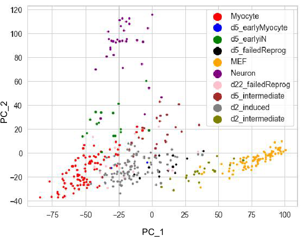
We first take a look at the PCA figure which shows the first 2 PCs of
the dataset. PCA is a linear methods which cannot reflect cell fate
differentation process.
Since the diffusion map applied the Gaussian kernal during the distances
calculation, it usually a better way to capture the cell differentation
events. Here we show diffusion dimension 1,2 and 1,3. It's clear that
1,2 captures the cell differentation from fibroblasts to neuron, and 1,3
captures the differentiation from firoblasts to myocytes.
We can change the bandwidth from 7 to 100, which use the 100th
neareast neighbor as bandwidth instead of 7th. The following shows the
diffusion map that bandwidth=100.
pseudo time by random walk
The eigenvalue decomposition of graph laplacian can also be used to
infer the pseudo time simulating the pseudo time of cell differentation
events. We here set top \(m\) cells
\(1/m\) of the progenitor cells (MEF)
and set other cell 0 as the initial state. Next, we perform random walk
to get new pesudotime \(u\) such that:
\[\begin{equation}
u = [\frac{1}{m}, \frac{1}{m}, \cdots, 0, \cdots 0](D^{-1}W)^t
\end{equation}\] By testing different number of random walk steps
we can check the new pseudo time \(u\).
Here we show time step equals to 1, 10, 100 and 200. From the figure we
can notice that after certain step, the pseudo time will not change
anymore. That means the random walk reaches the steady state.
To test when can we reach the steady state, I use the graph we
mentioned in my last post Spectral
analysis (1):
Here we random generate two initial states (\(v_1\), \(v_2\)) to do the random walk such that:
\[\begin{equation}
\begin{aligned}
v_1 &= [0.15,0.41,0.54,0.9,0.62,0.93,0.1,0.46,0.01,0.88]\\
v_2 &= [0.89,0.93,0.07,0.41,0.52,0.88,0.43,0.09,0.1,0.2]
\end{aligned}
\end{equation}\]
From the the figure below we can see that \(v_1\) reaches the steady state in 30 steps
whereas \(v_2\) reaches steady state in
100 steps. In total, all these two initial state will reach the steady
state that would not change any longer.
spectral clustering
The eigenvectors of graph Laplacian can also be used to do the
clustering. From the figure we can find clear cut using the 1st, 2nd and
the 3rd diffusion dimensions. In practice, we can use kmeans, DBSCAN,
leiden, louvain algorithm to perform clustering using the diffusion
dimensions.
R = np.array(R) if not sigma: s =[top_k(R[:, i], k=k)for i inrange(R.shape[1])] S = np.sqrt(np.outer(s, s)) else: S = sigma logW =-np.power(np.divide(R, S),2) iflog: return logW return np.exp(logW)
def diffusionMaps(R,k=7,sigma=None): """ Diffusion map(Coifman, 2005) https://en.wikipedia.org/wiki/Diffusion_map ---------- dic: psi: right eigvector of P = D^{-1/2} * evec phi: left eigvector of P = D^{1/2} * evec eig: eigenvalues """ k=k-1## k is R version minus 1 for the index logW = affinity(R,k,sigma,log=True) rs = np.exp([logsumexp(logW[i,:])for i inrange(logW.shape[0])])## dii=\sum_j w_{i,j} D = np.diag(np.sqrt(rs)) ## D^{1/2} Dinv = np.diag(1/np.sqrt(rs))##D^{-1/2} Ms = Dinv @ np.exp(logW)@ Dinv ## D^{-1/2} W D^{-1/2} e = np.linalg.eigh(Ms)## eigen decomposition of P' evalue= e[0][::-1] evec = np.flip(e[1], axis=1) s = np.sum(np.sqrt(rs)* evec[:,0])# scaling # Phi is orthonormal under the weighted inner product #0:Psi, 1:Phi, 2:eig dic ={'psi':s * Dinv@evec,'phi':(1/s)*D@evec,"eig": evalue} return dic
Newton used glass separted the white sunlight into red, orange,
yellow, green, blue, indigo and violet single colors. The light spectrum
analysis can help scientists to interpret the world. For example, we can
detect the elements of our solar system as well as far stars in the
universe. The spectrum analysis is also a field in mathmatjics. In the
graph thoery field, Laplacian matrix is used to represented a graph. We
can obtian features from the undirected graph below (wikipedia).
For example, we can check the degree of each vertex, which forms our
Degree matrix \(D\) such that: \[\begin{equation}
D = \begin{pmatrix}
2 & 0 & 0 & 0 & 0 & 0\\
0 & 3 & 0 & 0 & 0 & 0\\
0 & 0 & 2 & 0 & 0 & 0\\
0 & 0 & 0 & 3 & 0 &0\\
0 & 0 & 0 & 0 & 3 & 0\\
0 & 0 & 0 & 0 & 0 & 1
\end{pmatrix}
\end{equation}\]
By checking the connection between all pairs nodes, we can create a
Adjacency matrix:
In fact, the graph Laplaican matrix is symmetric and also positive
semidefinite (PSD), which means if we perform eigenvalue decomposition,
the eigen values are all real and nonnegative. We can normlize the graph
Laplaican by left multiplying the \(D^{-1}\) which will give rise to all \(1\)s of the diagnal entries of the matrix,
namely: \[\begin{equation}
\text{norm}({L}) = D^{-1}L = \begin{pmatrix}1 & -0.50 & 0
& 0 & -0.50 & 0\\
-0.33 & 1 & -0.33 & 0 & -0.33 & 0\\
0 & -0.50 & 1 & -0.50 & 0 & 0\\
0 & 0 & -0.33 & 1 & -0.33 &-0.33\\
-0.33 & -0.33 & 0 & -0.33 & 1 & 0\\
0 & 0 & 0 & -1 & 0 & 1
\end{pmatrix}
\end{equation}\] This matrix is called transition matrix.
However, the matrix would not keep the symmetric and the PSD property
after the normalization. We will come back to discuss the spectral for
the normalized graph Laplacian.
Weighted graph
In practice, graph are usually weighted. The weight between vertices
can be euclidean distance or other measures. The figure blow shows the
weights of the graph. Here we apply gussian kernel to the euclidean
distances between vertices such that:
\[\begin{equation}
w_{ij} =\exp (-r_{ij}^2/\sigma) = \exp \big(\frac{-\|x_i -
x_j\|^2}{\sigma_i\sigma_j}\big)
\end{equation}\] where \(r_{ij}\) is the euclidean distance between
vetex \(i\) and \(j\), and \(sigma\) controls the bandwidth. We call the
matrix \(W=(w_{ij})\) gaussian affinity
matrix such that: \[\begin{equation}
\begin{pmatrix}
0 & w_{12} & w_{13} & w_{14} & w_{15}& w_{16}\\
w_{21} & 0 & w_{23} & w_{24} & w_{25}& w_{26}\\
w_{31} & w_{32} & 0 & w_{34} & w_{35}& w_{36}\\
w_{41} & w_{42} & w_{43} & 0 & w_{45}& w_{46}\\
w_{51} & w_{52} & w_{53} & w_{54} & 0& w_{56}\\
w_{61} & w_{62} & w_{63} & w_{64} & w_{65}& 0
\end{pmatrix}
\end{equation}\] The guassian kernel would enlarge the distance
between too far vertices. Similar to unweighted matrix, we can also
construct graph Laplaican matrix using the gaussian affinity matrix.
First, we need find the weighted degree based on \(W\) such that: \[\begin{equation}
d_{ii} = \sum_j{w_{ij}}
\end{equation}\] With the diagnal degree matrix and affinity
matrix, we now can have the weighted laplacian that: \[\begin{equation}
L = D - W
\end{equation}\] Likewise, we next give the normalized form of
Laplacian such that: \[\begin{equation}
\text{norm}{(L)}= D^{-1}L = I - D^{-1}W
\end{equation}\] To facilitate the eigenvalue decomposition, we
need apply trick to the asymmetric matrix \(D^{-1}L\). Since the eigenvectors of \(D^{-1}L\) and \(D^{-1}W\) are the same, we apply some trick
to \(P = D^{-1}W\) to simplify the
problem. Lets construct \(P'\) such
that: \[\begin{equation}
P' = D^{1/2} P D^{-1/2} = D^{-1/2}WD^{-1/2}
\end{equation}\] It obvious \(P'\) is symmetric due to the
symmetrisation of \(W\). We can perform
eigenvalue decomposition on \(P'\)
such that: \[\begin{equation}
P' = S\Lambda S^\top
\end{equation}\] Where S stores the eigenvectors of \(P'\) and the diagonals of \(\Lambda\) records the eigenvalues of \(P'\). We can also get the decompostion
to \(P\) such that: \[\begin{equation}
P = D^{-1/2}S\Lambda S^\top D^{1/2}
\end{equation}\] Let \(Q=D^{-1/2}\), then \(Q^{-1}=S^{\top}D^{1/2}\). We therefore find
the right and left eigenvector of \(P\)
such that: \[\begin{equation}
\psi = D^{-1/2} S \qquad
\phi = S^{\top}D^{1/2}
\end{equation}\] In fact, columns of \(\psi\) stores the spectral of the graph
which also call diffusion map dimensions.
#Torch.nn.Linear y = x A^T + b torch.manual_seed(42) linear = torch.nn.Linear(in_features=2, # in_features = matches inner dimension of input out_features=6) # out_features = describes outer value x = tensor_A output = linear(x) x.shape, output, output.shape
other operations
1 2 3 4 5 6 7 8 9 10 11 12
tensor = torch.arange(10, 100, 10) # tensor([10, 20, 30, 40, 50, 60, 70, 80, 90]) tensor.argmax() # 8 tensor.argmin() # 0 tensor.type(torch.float16) # tensor([10., 20., 30., 40., 50., 60., 70., 80., 90.] torch.reshape(new_shape) # -1 is to ask calculating automatically tensor.view(new_shape) # return a new shape view torch.stack(t, dim=0) # concate a sequence of tensors along a new dimension(dim) torch.squeeze() # all into the first dimensions torch.clamp() # min=min, max=max, limit the range torch.unsqueeze() torch.permute() # torch.Size([224, 224, 3]) -> torch.Size([3, 224, 224]) torch.permute_(), x.unsqueeze_() -> inplace operation
random seed torch.manual_seed(seed=RANDOM_SEED) torch.random.manual_seed(seed=RANDOM_SEED)
Variable
1 2 3 4 5 6 7 8 9 10
torch.autograd import Variable .data, .grad, .grad_fn x_tensor = torch.randn(10, 5) y_tensor = torch.randn(10, 5) x = Variable(x_tensor, requires_grad=True) y = Variable(y_tensor, requires_grad=True) z = torch.sum(x + y) print(z.data) #-2.1379 print(z.grad_fn) #<SumBackward0 object at 0x10da636a0> z.backward()
GPU
1
2
3
4
5
6
7
8
9
if torch.cuda.is_available(): device = "cuda"# Use NVIDIA GPU (if available) elif torch.backends.mps.is_available(): device = "mps"# Use Apple Silicon GPU (if available) else: device = "cpu"# Default to CPU if no GPU is available
tensor.to(device) tensor_on_gpu.cpu().numpy()
Neural network
torch.nn
Contains all of the building blocks for computational graphs
(essentially a series of computations executed in a particular way).
torch.nn.Parameter
Stores tensors that can be used with nn.Module. If requires_grad=True
gradients (used for updating model parameters via gradient descent) are
calculated automatically, this is often referred to as "autograd".
torch.nn.Module
The base class for all neural network modules, all the building
blocks for neural networks are subclasses. If you're building a neural
network in PyTorch, your models should subclass nn.Module. Requires a
forward() method be implemented.
torch.optim
Contains various optimization algorithms (these tell the model
parameters stored in nn.Parameter how to best change to improve gradient
descent and in turn reduce the loss).
def forward()
All nn.Module subclasses require a forward() method, this defines the
computation that will take place on the data passed to the particular
nn.Module (e.g. the linear regression formula above).
loss_fn = nn.L1Loss() # MAE loss is same as L1Loss optimizer = torch.optim.SGD(params=model_0.parameters(), lr=0.01) ## lr(learning rate)
Step name
What does it do?
Code example
1
Forward pass
The model goes through all of the training data once, performing its
forward() function calculations.
model(x_train)
2
Calculate the loss
The model's outputs (predictions) are compared to the ground truth
and evaluated to see how wrong they are.
loss = loss_fn(y_pred, y_train)
3
Zero gradients
The optimizers gradients are set to zero (they are accumulated by
default) so they can be recalculated for the specific training
step.
optimizer.zero_grad()
4
Perform backpropagation on the loss
Computes the gradient of the loss with respect for every model
parameter to be updated (each parameter with requires_grad=True)
loss.backward()
5
Update the optimizer (gradient descent)
Update the parameters with requires_grad=True with respect to the
loss gradients in order to improve them.
optimizer.step()
Training example
1 2 3 4 5 6 7
for epoch inrange(epoches): model.train() y_pred = model(X_train) loss = loss_fn(y_pred, y_true) optimizer.zero_grad() loss.backward() optimizer.step()
test
Forward pass
The model goes through all of the training data once, performing its
forward() function calculations.
model(x_test)
Calculate the loss
The model's outputs (predictions) are compared to the ground truth
and evaluated to see how wrong they are.
loss = loss_fn(y_pred, y_test)
Calulate evaluation metrics (optional)
Alongisde the loss value you may want to calculate other evaluation
metrics such as accuracy on the test set.
Custom functions
Inference and save model
Inferennce
model_0.eval() # Set the model in evaluation mode with
torch.inference_mode(): y_preds = model_0(X_test)
torch.save
Saves a serialized object to disk using Python's pickle utility.
Models, tensors and various other Python objects like dictionaries can
be saved using torch.save.
torch.load
Uses pickle's unpickling features to deserialize and load pickled
Python object files (like models, tensors or dictionaries) into memory.
You can also set which device to load the object to (CPU, GPU etc).
torch.nn.Module.load_state_dict ## recommended
Loads a model's parameter dictionary (model.state_dict()) using a
saved state_dict() object.
torch.manual_seed(42) epochs = 100# Set the number of epochs
# Create empty loss lists to track values train_loss_values = [] test_loss_values = [] epoch_count = []
for epoch inrange(epochs): ### Training model_0.train() # Put model in training mode (this is the default state of a model)
# 1. Forward pass on train data using the forward() method inside y_pred = model_0(X_train) # 2. Calculate the loss (how different are our models predictions to the ground truth) loss = loss_fn(y_pred, y_train) optimizer.zero_grad() # 3. Zero grad of the optimizer loss.backward() # 4. Loss backwards optimizer.step() # 5. Progress the optimizer ### Testing # Put the model in evaluation mode model_0.eval()
with torch.inference_mode(): # 1. Forward pass on test data test_pred = model_0(X_test)
# 2. Caculate loss on test data # predictions come in torch.float datatype, so comparisons need to be done with tensors of the same type test_loss = loss_fn(test_pred, y_test.type(torch.float))
# Print out what's happening if epoch % 10 == 0: epoch_count.append(epoch) train_loss_values.append(loss.detach().numpy()) test_loss_values.append(test_loss.detach().numpy()) print(f"Epoch: {epoch} | MAE Train Loss: {loss} | MAE Test Loss: {test_loss} ")
# Put data on the available device # Without this, error will happen (not all model/data on device) X_train = X_train.to(device) X_test = X_test.to(device) y_train = y_train.to(device) y_test = y_test.to(device)
for epoch inrange(epochs): ### Training model_1.train() # train mode is on by default after construction
# 1. Forward pass y_pred = model_1(X_train) # 2. Calculate loss loss = loss_fn(y_pred, y_train)
# 3. Zero grad optimizer optimizer.zero_grad()
# 4. Loss backward loss.backward()
# 5. Step the optimizer optimizer.step()
### Testing model_1.eval() # put the model in evaluation mode for testing (inference) # 1. Forward pass with torch.inference_mode(): test_pred = model_1(X_test)
# 2. Calculate the loss test_loss = loss_fn(test_pred, y_test)
if epoch % 100 == 0: print(f"Epoch: {epoch} | Train loss: {loss} | Test loss: {test_loss}")
# Create a neural net class classNet(nn.Module): # Constructor def__init__(self, num_classes=3): super(Net, self).__init__()
# Our images are RGB, so input channels = 3. We'll apply 12 filters in the first convolutional layer self.conv1 = nn.Conv2d(in_channels=3, out_channels=12, kernel_size=3, stride=1, padding=1)
# We'll apply max pooling with a kernel size of 2 self.pool = nn.MaxPool2d(kernel_size=2)
# A second convolutional layer takes 12 input channels, and generates 12 outputs self.conv2 = nn.Conv2d(in_channels=12, out_channels=12, kernel_size=3, stride=1, padding=1)
# A third convolutional layer takes 12 inputs and generates 24 outputs self.conv3 = nn.Conv2d(in_channels=12, out_channels=24, kernel_size=3, stride=1, padding=1)
# A drop layer deletes 20% of the features to help prevent overfitting self.drop = nn.Dropout2d(p=0.2) # Our 128x128 image tensors will be pooled twice with a kernel size of 2. 128/2/2 is 32. # So our feature tensors are now 32 x 32, and we've generated 24 of them # We need to flatten these and feed them to a fully-connected layer # to map them to the probability for each class self.fc = nn.Linear(in_features=32 * 32 * 24, out_features=num_classes)
defforward(self, x): # Use a relu activation function after layer 1 (convolution 1 and pool) x = F.relu(self.pool(self.conv1(x)))
# Use a relu activation function after layer 2 (convolution 2 and pool) x = F.relu(self.pool(self.conv2(x)))
# Select some features to drop after the 3rd convolution to prevent overfitting x = F.relu(self.drop(self.conv3(x)))
# Only drop the features if this is a training pass x = F.dropout(x, training=self.training)
# Flatten x = x.view(-1, 32 * 32 * 24) # Feed to fully-connected layer to predict class x = self.fc(x) # Return log_softmax tensor return F.log_softmax(x, dim=1)
import torch import torch.autograd as autograd import torch.nn as nn import torch.functional as F import torch.optim as optim from torch.nn.utils.rnn import pack_padded_sequence, pad_packed_sequence
Suppose we have two sets of variable corresponding to two aspects
such as height and weight, we want to analysis the relationship between
this two sets. There are several ways to measure the relationship
between them. However, sometime the it is hard to handle datasets with
different dimensions, meaning, if \(X\in
\mathbb{R}^m\) and \(Y\in
\mathbb{R}^n\), how to resolve the relationship?
basic of CCA
Assume there are two sets of data \(X\) and \(Y\), the size of \(X\) is \(n \times
p\), whereas size of \(Y\) is
\(n\times q\). That is, \(X\) and \(Y\) share the same row numbers but are
differnt in columns number. The idea of CCA is simple: find the best
match of \(X w_x\) and \(Y w_y\). Let's just set: \[X w_x = z_x\qquad\text{and}\qquad Y w_y =
z_y\]
Where \(X\in \mathbb{R}^{n\times
p}\), \(w_x \in
\mathbb{R}^{p}\), \(z_x\in
\mathbb{R}^n\), \(Y\in
\mathbb{R}^{n\times q}\), \(w_y \in
\mathbb{R}^{q}\), \(z_y\in
\mathbb{R}^n\). \(w_x\) and
\(w_y\) are often refered as canonical
weight vectors, \(z_x\) and \(z_y\) are named images as well as canonical
variates or canonical scores. To simplify the problem, we assume \(X\) and \(Y\) are standardized to zero mean and unit
variance. Our task is to maximize the angle of \(z_x\) and \(z_y\), meaning:
with respect to: \(\|z_x\|_{2}=1\quad
\|z_y\|_{2}=1\).
In fact, our task is just project \(X\) and \(Y\) to a new coordinate system after the
linear transformation to \(X\) and
\(Y\).
Resolve CCA
There are many solutions to this problems. Before start, We need make
some assumptions: 1. the each column vector of \(X\) is perpendicular to the others. Which
means \(X^T X= I\). The assumption is
the same with \(Y\) and \(w_x, w_y\). We can find \(\min(p,q)\) canonical components, and the
\(r\)th component is orthogonal to all
the \(r-1\) components.
Resolve CCA through SVD
To solve the CCA problem using SVD, we first introduce the joint
covariance matrix \(C\) such such that:
\[\begin{equation}
C = \begin{pmatrix}
C_{xx} & C_{xy}\\
C_{yx} & C_{yy}\\
\end{pmatrix}
\end{equation}\] Where \(C_{xx}=\frac{1}{n-1}X^\top X\) and \(C_{yy}=\frac{1}{n-1}Y^\top Y\) are the
empirical variance matrices between \(X\) and \(Y\) respectively. The \(C_{xy}=\frac{1}{n-1} X^\top Y\) is the
covariance matrix between \(X\) and
\(Y\).
We next can reform CCA problem with two linear transformations \(w_x\) and \(w_y\) such that:
\[\begin{equation}
w_x^\top C_{xx} w_x = I_p, \quad w_y^\top C_{yy} w_y = I_q, \quad
w_x^\top C_{xy} w_y = D
\end{equation}\] Where I_p and I_q are th p-dimensional and
q-dimensional identity meatrics respectively. The diagonal matrix \(D = \text{diag}(\gamma_i)\) so that:
The canoical variable: \[\begin{equation}
Z_x = Xw_x, \quad Z_y = Y w_y
\end{equation}\] The diagonal elements \(\gamma_i\) of D denote the canonical
correlations. Thus we find the linear compounds \({Z}_x\) and \({Z}_y\) to maximize the cross-correlations.
Since both \(C_{xx}\) and \(C_{yy}\) are symmetric positive definite,
we can perform Cholesky Decomposition on them to get: \[\begin{equation}
C_{xx} = C_{xx}^{\top/2} C_{xx}^{1/2}, \quad C_{yy} =
C_{yy}^{\top/2} C_{yy}^{1/2}
\end{equation}\]
where \(C_{xx}^{\top/2}\) is the
transpose of \(C_{xx}^{1/2}\). Applying
the inverses of the square root factors symmetrically on the joint
covariance matrix \(C\), the matrix is
transformed into: \[\begin{equation}
\begin{pmatrix}
C_{xx}^{-\top/2} & {\mathbf 0}\\
{\mathbf 0} & C_{yy}^{-\top/2}
\end{pmatrix}
\begin{pmatrix}
C_{xx} & C_{ab}\\
C_{yx} & C_{yy}
\end{pmatrix}
\begin{pmatrix}
C_{xx}^{-1/2} & {\mathbf 0}\\
{\mathbf 0} & C_{yy}^{-1/2}
\end{pmatrix}
=
\begin{pmatrix}
I_p & C_{xx}^{-1/2}C_{ab}C_{yy}^{-1/2}\\
C_{yy}^{-1/2}C_{yx}C_{xx}^{-1/2} & I_q
\end{pmatrix}.
\end{equation}\]
The canonical correlation problem is reduced to that of finding an
SVD of a triple product: \[\begin{equation}
U^{\top} (C_{xx}^{-1/2}C_{ab}C_{yy}^{-1/2}) V = D.
\end{equation}\] The matrix \(C\) is thus reduced to the joint covariance
matrix by applying a two-sided Jacobi method such that: \[\begin{equation}
\begin{pmatrix}
U^\top & {\mathbf 0}\\
{\mathbf 0} & V^\top
\end{pmatrix}
\begin{pmatrix}
I_p & C_{xx}^{-1/2}C_{ab}C_{yy}^{-1/2}\\
C_{yy}^{-1/2}C_{_y}C_{xx}^{-1/2} & I_q
\end{pmatrix}
\begin{pmatrix}
U & {\mathbf 0}\\
{\mathbf 0} & V
\end{pmatrix} =
\begin{pmatrix}
I_p & D\\
D^\top & I_q
\end{pmatrix}
\end{equation}\]
with the desired transformation \({w}_x\) and \({w}_y\): \[\begin{equation}
{w}_x = C_{xx}^{-1/2} U, \quad {w}_y = C_{yy}^{-1/2}V
\end{equation}\] where the singular values \(\gamma_i\) are in descending order such
that: \[\begin{equation}
\gamma_1 \geq \gamma_2 \geq \cdots \geq 0.
\end{equation}\]
Resolve CCA
through Standard EigenValue Problem
The Problem can be reformed to solve the problem: \[\begin{equation}
\underset{w_x \in \mathbb{R}^p, w_y\in \mathbb{R}^q}{\arg \max} w_x^\top
C_{xy} w_y
\end{equation}\] With respect to \(\|\|w_x^\top C_{xx} w_x\|\|_2 = \sqrt{w_x^\top
C_{xx} w_x}=1\) and \(\|\|w_y^\top
C_{yy} w_y\|\|_2 = \sqrt{w_y^\top C_{yy} w_y}=1\). The problem
can apparently sovled by Lagrange multiplier technique. Let construct
the Lagrange multiplier \(L\) such
that: \[\begin{equation}
L = w_x^\top C_{xy} w_y - \frac{\rho_1}{2} w_x^\top C_{xx} w_x -
\frac{\rho_2}{2} w_y^\top C_{yy} w_y
\end{equation}\]
The differentiation of L to \(w_x\)
and \(w_y\) is: \[\begin{equation}
\begin{aligned}
\frac{\partial L}{\partial w_x} = C_{xy} w_y - \rho_1 C_{xx}w_x =
\mathbf{0}\\
\frac{\partial L}{\partial w_y} = C_{yx} w_x - \rho_2 C_{yy}w_y =
\mathbf{0}
\end{aligned}
\end{equation}\]
By left multipling \(w_x\) and \(w_y\) the above equation, we have:
\[\begin{equation}
\begin{aligned}
w_x^\top C_xy w_y -\rho_1 w_x^\top C_xx w_x = \mathbf{0}\\
w_y^\top C_yx w_x -\rho_2 w_y^\top C_yy w_y = \mathbf{0}
\end{aligned}
\end{equation}\] Since w_x^C_xx w_x = 1 and w_y^C_yy w_y = 1, we
can obtain that \(\rho_1 = \rho_2 =
\rho\). By substituting \(\rho\)
to the formula. We can get: \[\begin{equation}
w_x = \frac{C_{xx}^{-1}C_{xy}w_y}{rho}
\end{equation}\] Evantually we have the equation: \[\begin{equation}
C_{yx} C_{xx}^{-1} C_{xy} w_y = \rho^2 C_yy w_y
\end{equation}\] Obviously, this is the form of eigenvalue
decompostion problem where all eigen values are greater or equal to
zero. By solving the eigenvalue decomposition we can find \(w_x\) and \(w_y\).
INFO  Start processing
FATAL Something's wrong. Maybe you can find the solution here: http://hexo.io/docs/troubleshooting.html
Template render error: (unknown path) [Line 65, Column 565]
  expected variable end
    at Object._prettifyError (/Users/chengmingbo/blog_deploy/blog/node_modules/nunjucks/src/lib.js:36:11)
    at Template.render (/Users/chengmingbo/blog_deploy/blog/node_modules/nunjucks/src/environment.js:542:21)
    at Environment.renderString (/Users/chengmingbo/blog_deploy/blog/node_modules/nunjucks/src/environment.js:380:17
    ... ...
Our aim is to derive the the expectation of \(E(X)\) and the variance \(Var(X)\). Given that the formula of
expectation: \[
E(X)=\sum_{k=0}^{\infty} k \frac{\lambda^k e^{-\lambda }}{k!}
\]
Notice that when \(k=0\), the
formula is equal to 0, that is:
\[\sum_{k=0}^{\infty} k
\frac{\lambda^ke^{-\lambda}}{k!}\Large|_{k=0}=0\]
Then, the formula become as followed:
\[E(X)=\sum_{k=1}^{\infty} k
\frac{\lambda^ke^{-\lambda}}{k!}\]
\[\begin{aligned}E(X)&=\sum_{k=0}^{\infty} k
\frac{\lambda^ke^{-\lambda}}{k!}=\sum_{k=0}^{\infty}
\frac{\lambda^ke^{-\lambda}}{(k-1)!}\\&=\sum_{k=0}^{\infty} \frac{\lambda^{k-1}\lambda
e^{-\lambda}}{(k-1)!}\\&=\lambda
e^{-\lambda}\sum_{k=1}^{\infty}\frac{\lambda^{k-1}}{(k-1)!}\end{aligned}\]
Now we need take advantage of Taylor Expansion, recall that:
As known that \(Var(X)=E(X^2)-(E(x))^2\), we just get \(E(X^2)\). Given that:
\[E(X)=\sum_{k=1}^{\infty} k
\frac{\lambda^ke^{-\lambda}}{k!}=\lambda\]
we can use this formula to derive the \(E(X^2)\),
\[\begin{aligned}E(X)=&\sum_{k=1}^{\infty} k
\frac{\lambda^ke^{-\lambda}}{k!}=\lambda\\\Leftrightarrow&\sum_{k=1}^{\infty}
k \frac{\lambda^k}{k!}=\lambda
e^{\lambda}\\\Leftrightarrow&\frac{\partial\sum_{k=1}^{\infty} k
\frac{\lambda^k}{k!}}{\partial \lambda}=\frac{\partial \lambda
e^{\lambda}}{\partial
\lambda}\\\Leftrightarrow&\sum_{k=1}^{\infty}k^2\frac{\lambda^{k-1}}{k!}=e^\lambda+\lambda
e^\lambda\\\Leftrightarrow&\sum_{k=1}^{\infty}k^2\frac{\lambda^{k-1}e^{-\lambda}}{k!}=1+\lambda
\\\Leftrightarrow&\sum_{k=1}^{\infty}k^2\frac{\lambda^{k}e^{-\lambda}}{k!}=\lambda+\lambda^2=E(X^2)\end{aligned}\]
There are many classification algorithm such as Logistic Regression,
SVM and Decision Tree etc. Today we'll talk about Gaussian Discriminant
Analysis(GDA) Algorithm, which is not so popular. Actually, Logistic
Regression performance better than GDA because it can fit any
distributions from exponential family. However, we can learn more
knowledge about gaussian distribution from the algorithm which is the
most import distribution in statistics. Furthermore, if you want to
understand Gaussian Mixture Model or Factor Analysis, GDA is a good
start.
We, firstly, talk about Gaussian Distribution and Multivariate
Gaussian Distribution, in which section, you'll see plots about Gaussian
distributions with different parameters. Then we will learn GDA
classification algorithm. We'll apply GDA to a dataset and see the
consequnce of it.
Multivariate Gaussian
Distribution
Gaussian Distribution
As we known that the pdf(Probability Distribution Function) of
gaussian distribution is a bell-curve, which is decided by two
parameters \(\mu\) and \(\sigma^2\). The figure below shows us a
gaussian distribution with \(\mu=0\)
and \(\sigma^2=1\), which is often
referred to \(\mathcal{N}(\mu,
\sigma^2)\). Thus, Figure1 is distributed normally with \(\mathcal{N}(0,1)\).
Figure 1. Gaussian Distribution with \(\mu=0\) and \(\sigma^2=1\).
Actually, parameter \(\mu\) and
\(\sigma^2\) are exactly the mean and
the variance of the distribution. Therefore, \(\sigma\) is the stand deviation of normal
distribution. Let's take a look at area between red lines and magenta
lines, which are respectively range from \(\mu\pm\sigma\) and from \(\mu\pm2\sigma\). The area between redlines
accounts for 68.3% of the total area under the curve. That is, there are
68.3% samples are between \(\mu-\sigma\) and \(\mu+\sigma\) . Likely, there are 95.4%
samples are between \(\mu-2\sigma\) and
\(\mu+2\sigma\).
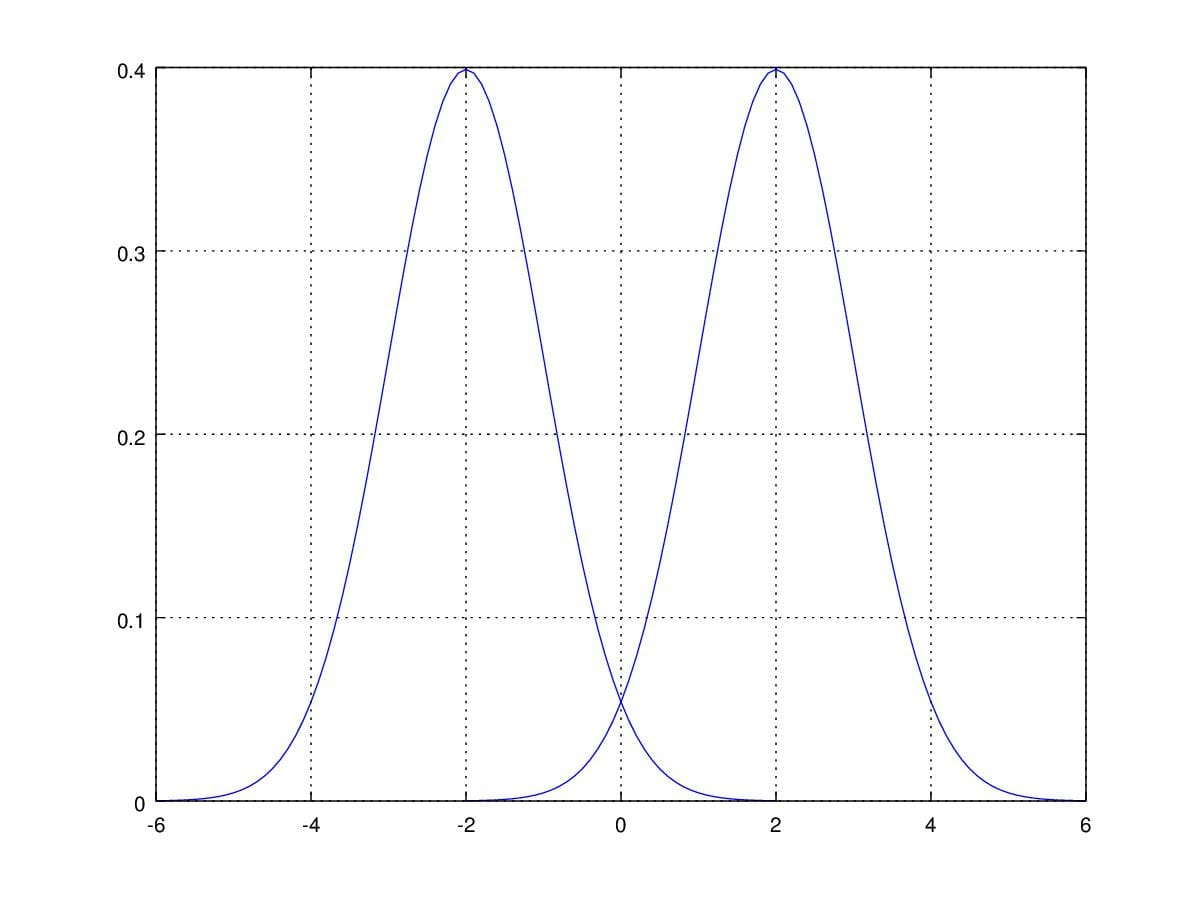
You must want to know how these two parameter influence the shape of
PDF of gaussian distribution. First of all, when we change \(\mu\) with fixed \(\sigma^2\), the curve is the same as before
but move along the random variable axis.
Figure 2. Probability Density Function curver with \(\mu=\pm2\) and \(\sigma=1\).
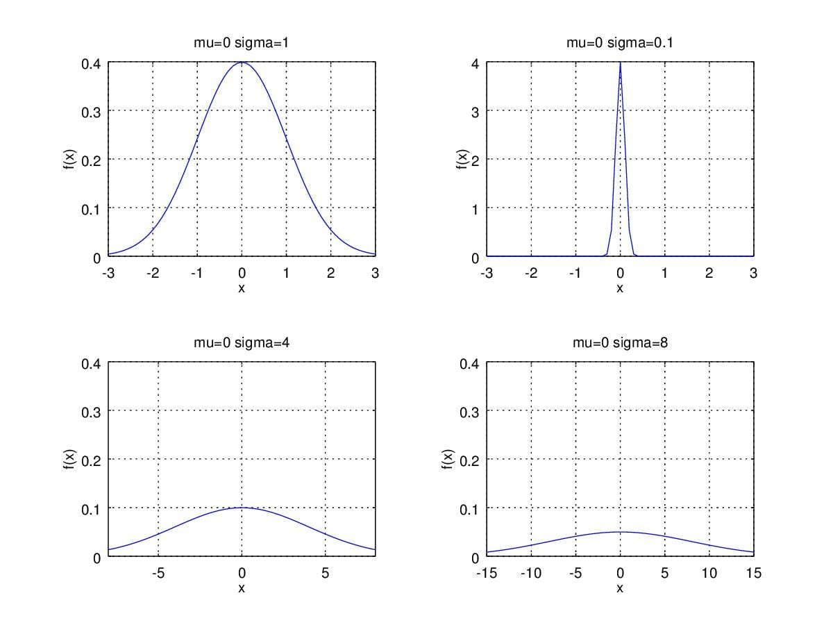
So, what if when we change \(\sigma\) then? Figure3. illustrates that
smaller \(\sigma\) lead to sharper
shape of pdf. Conversely, larger \(\sigma\) brings us broader curves.
Figure 3. Probability Density Function curver with \(\mu=0\) and change \(\sigma\).
Some may wonder what is the form of \(p(x)\) of a gaussian distribution, I just
demonstrate here, you can compare Normal distribution with Multivariate
Gaussian.
where \(\mu\) is the mean, \(\Sigma\) is the covariance matrices, \(d\) is the dimension of random variable
\(x\), specfically, 2-dimensional
gaussian distribution, we have:
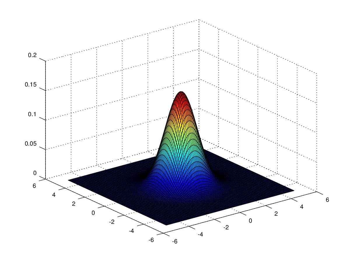
In order to get an intuition of Multivariate Guassian Distribution,
We first take a look at a distribution with \(\mu=\begin{pmatrix}0\\0\end{pmatrix}\) and
\(\Sigma=\begin{pmatrix}1&0\\0&1\end{pmatrix}\).
Figure 4. 2-dimensional gaussian distribution with \(\mu=\begin{pmatrix}0\\0\end{pmatrix}\) and
\(\Sigma=\begin{pmatrix}1&0\\0&1\end{pmatrix}\).
Notice that the the figure is rather than a curve but a 3-dimensional
diagram. Just like normal distribution pdf, \(\sigma\) determines the shape of the
figure. However, there are 4 entries of \(\Sigma\) can be changed in this example.
Given that we need compute \(|\Sigma|\)
as denominator and \(\Sigma^{-1}\)
which demands non-zero determinant of \(\Sigma\), we must keep in mind that \(|\Sigma|\) is positive.
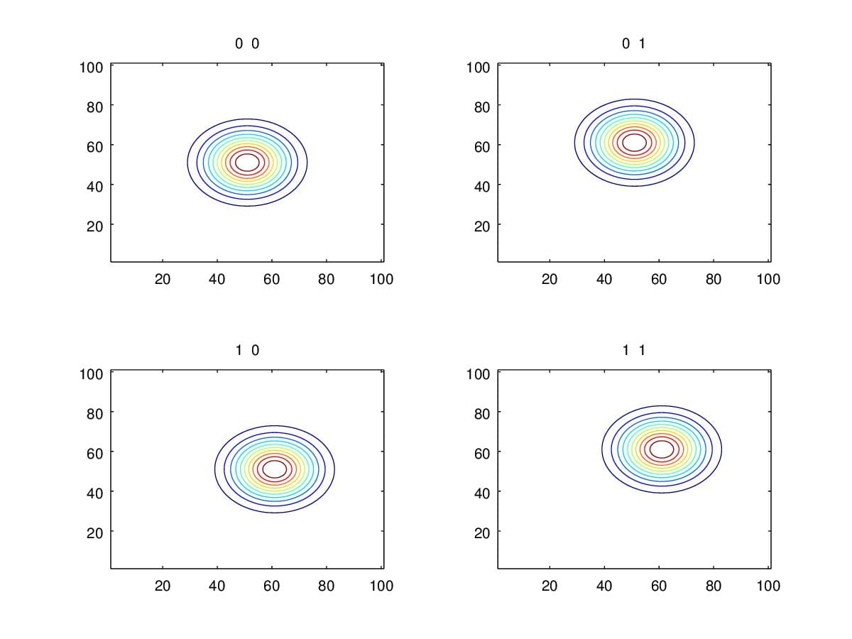
1. change \(\mu\)
Rather than change \(\Sigma\), we
firstly take a look at how the contour looks like when changing \(\mu\). Figure 5. illustrates the contour
variation when changing \(\mu\). As we
can see, we only move the center of the contour during the variation of
\(\mu\). i.e. \(\mu\) detemines the position of pdf rather
than the shape. Next, we will see how entries in \(\Sigma\) influence the shape of pdf.
Figure 5. Contours when change \(\mu\) with \(\Sigma=\begin{pmatrix}1&0\\0&1\end{pmatrix}\).
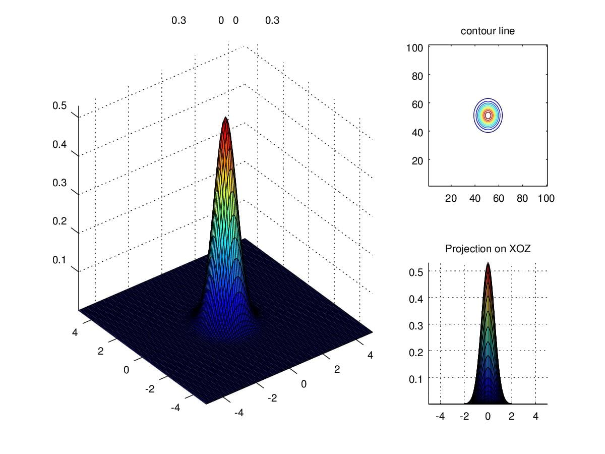
2. change diagonal entries of
\(\Sigma\)
If scaling diagonal entries, we can see from figure 6. samples are
concentrated to a smaller range when change \(\Sigma\) from \(\begin{pmatrix}1&0\\0&1\end{pmatrix}\)
to \(\begin{pmatrix}0.3&0\\0&0.3\end{pmatrix}\).
Similarly, if we alter \(\Sigma\) to
\(\begin{pmatrix}3&0\\0&3\end{pmatrix}\),
then figure will spread out.
Figure 6. Density when scaling diagonal entries to 0.3.
What if we change only one entry of the diagonal? Figure 7. shows the
variation of the density when change \(\Sigma\) to \(\begin{pmatrix}1&0\\0&5\end{pmatrix}\).
Notice the parameter spuashes and stretches the figure along coordinate
axis.
Figure 7. Density when scaling one of the diagonal entries.
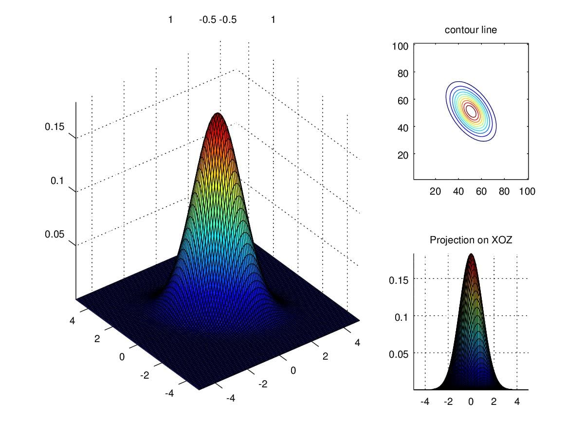
3. change secondary
diagonal entries of \(\Sigma\)
We now try to change entries along secondary diagonal. Figure 8.
demonstrates that the variation of density is no longer parallel to
\(X\) and \(Y\) axis, where \(\Sigma=\begin{pmatrix}1
&0.5\\0.5&1\end{pmatrix}\).
Figure 8. Density when scaling secondary diagonal entries to 0.5
When we alter secondary entries to negative 0.5, the direction of
contour presents a mirror to contour when positive.
Figure 9. Density when scaling secondary diagonal entries to -0.5
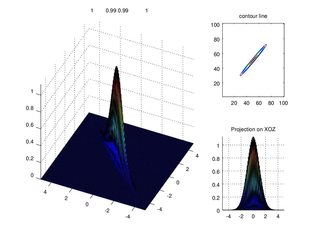
In light of the importance of determinant of \(\Sigma\), what will happen if the
determinant is close to zero. Actually, we can, informally, take
determinant of a matrice as the volume of which. Similarly, when
determinant is smaller, the volume under density curve become smaller.
Figure 10. illustrates the circumstance we talked above where \(\Sigma=\begin{pmatrix}1&0.99\\0.99&1\end{pmatrix}\).
Figure 10. Density when determinant is close to zero.
Gaussian Discriminant
Analysis
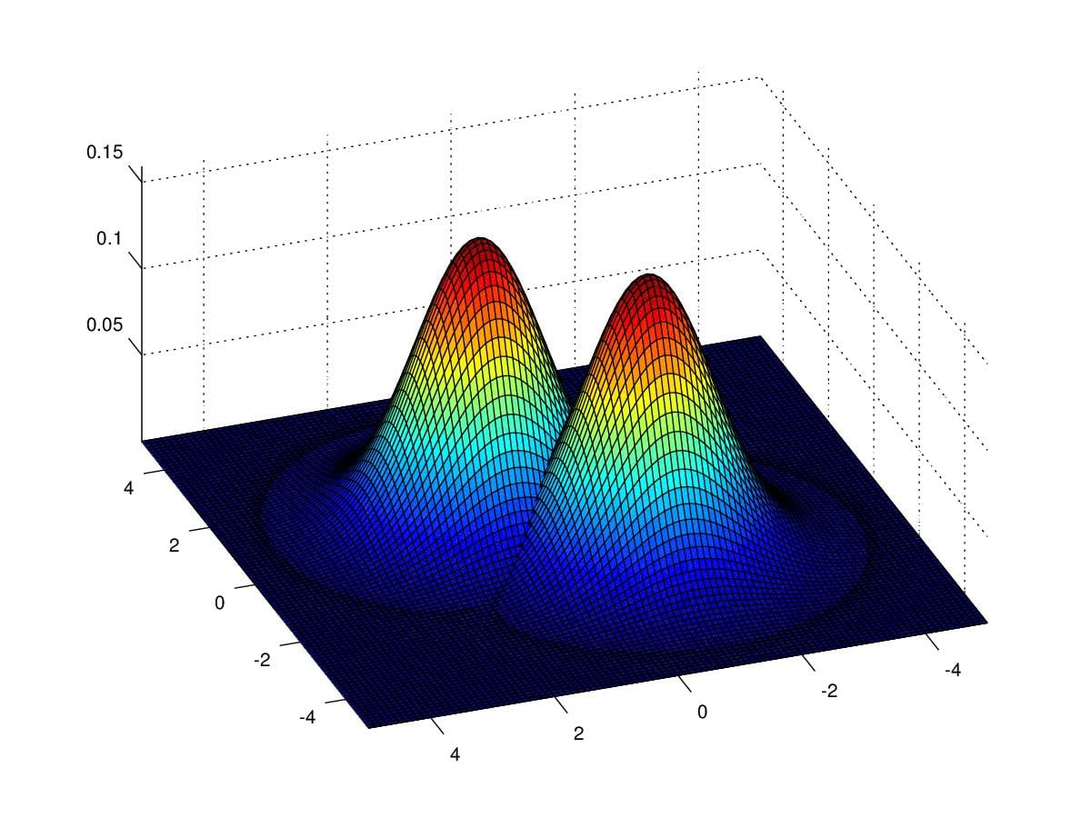
Intuition
When input features \(x\) are
continuous variables, we can use GDA classify data. Firstly, let's take
a look at how GDA to do the job. Figure 11. show us two gaussian
distributions, they share the same covariance \(\Sigma=\begin{pmatrix}1&0\\0&1\end{pmatrix}\)
, and repectively with parameter \(\mu_0=\begin{pmatrix}1\\1\end{pmatrix}\)
and \(\mu_1=\begin{pmatrix}-1\\-1\end{pmatrix}\).
Imagine you have some data which fall into the cover of the first and
second Gaussian Distribution. If we can find such distributions to fit
the data, then we'll have the capcity to decide which is new data coming
from, the first or the second one.
Figure 11. Two gaussian distributions with respect to \(\mu_0=\begin{pmatrix}1\\1\end{pmatrix}\)
and \(\mu_1=\begin{pmatrix}-1\\-1\end{pmatrix}\)
, and \(\Sigma=\begin{pmatrix}1&0\\0&1\end{pmatrix}\)
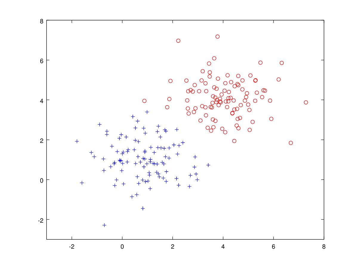
Specifically, let's look at a concrete example, Figure 12 are samples
drawn from two Gaussian distribution. There are 100 blue '+'s and 100
red 'o's. Assume that we have such data to be classified. We can apply
GDA to solve the problem.
Figure 12. 200 samples drawn from two Gaussian Distribution with
parameters \(\mu_0=\begin{bmatrix}1\\1\end{bmatrix},\mu_1=\begin{bmatrix}4\\4\end{bmatrix},\Sigma=\begin{bmatrix}1&0\\0&1\end{bmatrix}\).
Definition
Now, let's define the algorithm. Firstly we assume discrete random
variable classes \(y\) are distributed
Bernoulli and parameterized by \(\phi\), then we have:
\[y\sim {\rm Bernoulli}(\phi)\]
Concretely, the probablity of \(y=1\) is \(\phi\), and \(1-\phi\) when \(y=0\). We can simplify two equations to
one:
\(p(y|\phi)=\phi^y(1-\phi)^{1-y}\)
Apparently, \(p(y=1|\phi)=\phi\) and
\(p(y=0|\phi)=1-\phi\) given that y can
only be \(0\) or \(1\).
Another assumption is that we consider \(x\) are subject to different Gaussian
Distributions given different \(y\). We
assume the two Gaussian distributions share the same covariance and
different \(\mu\). Based on above all,
then
i.e. \(x|y=0 \sim
\mathcal{N}(\mu_0,\Sigma)\) and \(x|y=1
\sim \mathcal{N}(\mu_1,\Sigma)\). suppose we have \(m\) samples, it is hard to compute \(p(x^{(1)}, x^{(2)},
x^{(3)},\cdots,x^{(m)}|y=0)\) or \(p(x^{(1)}, x^{(2)},
x^{(3)},\cdots,x^{(m)}|y=1)\) . In general, we assume the
probabilty of \(x^{(i)}\)\(p(x^{(i)}|y=0)\) is independent to any
\(p(x^{(j)}|y=0)\), then we have:
Here \(X=(x^{(1)}, x^{(2)},
x^{(3)},\cdots,x^{(m)})\). Now, we want to maximize \(p(X|y=0)\) and \(p(X|y=1)\). Why is that, because we hope
find parameters that let \(p(X|y=0)p(X|y=1)\) largest, based on that
the samples are from the two Gaussian Distributions. These samples we
have are more likely emerging. Thus, our task is to maximize \(p(X|y=0)p(X|y=1)\) , we let
It's tough for us to maximize \(\mathcal{L}(\phi,\mu_0,\mu_1,\Sigma)\).
Notice function \(\log\) is monotonic
increasing. Thus, we can maximize \(\log\mathcal{L}(\phi,\mu_0,\mu_1,\Sigma)\)
instead of \(\mathcal{L}(\phi,\mu_0,\mu_1,\phi)\),
then:
By now, we have found a convex function with respect parameters \(\mu_0, mu_1,\Sigma\) and \(\phi\). Next section, we'll obtain these
parameter through partial derivative.
Solution
To estimate these four parameters, we just apply partial derivative
to \(\ell\). Now we estimate \(\phi\) in the first place. We let \(\frac{\partial \ell}{\partial \phi}=0\),
then
Before calculate \(\Sigma\), I first
illustrate the truth that \(\frac{\partial|\Sigma|}{\partial\Sigma}=|\Sigma|\Sigma^{-1},\quad
\frac{\partial\Sigma^{-1 } } {\partial\Sigma}=-\Sigma^{-2}\),
then
In spite of the harshness of the deducing, the outcome are pretty
beautiful. Next, we will apply these parameters and see how the
estimation performance.
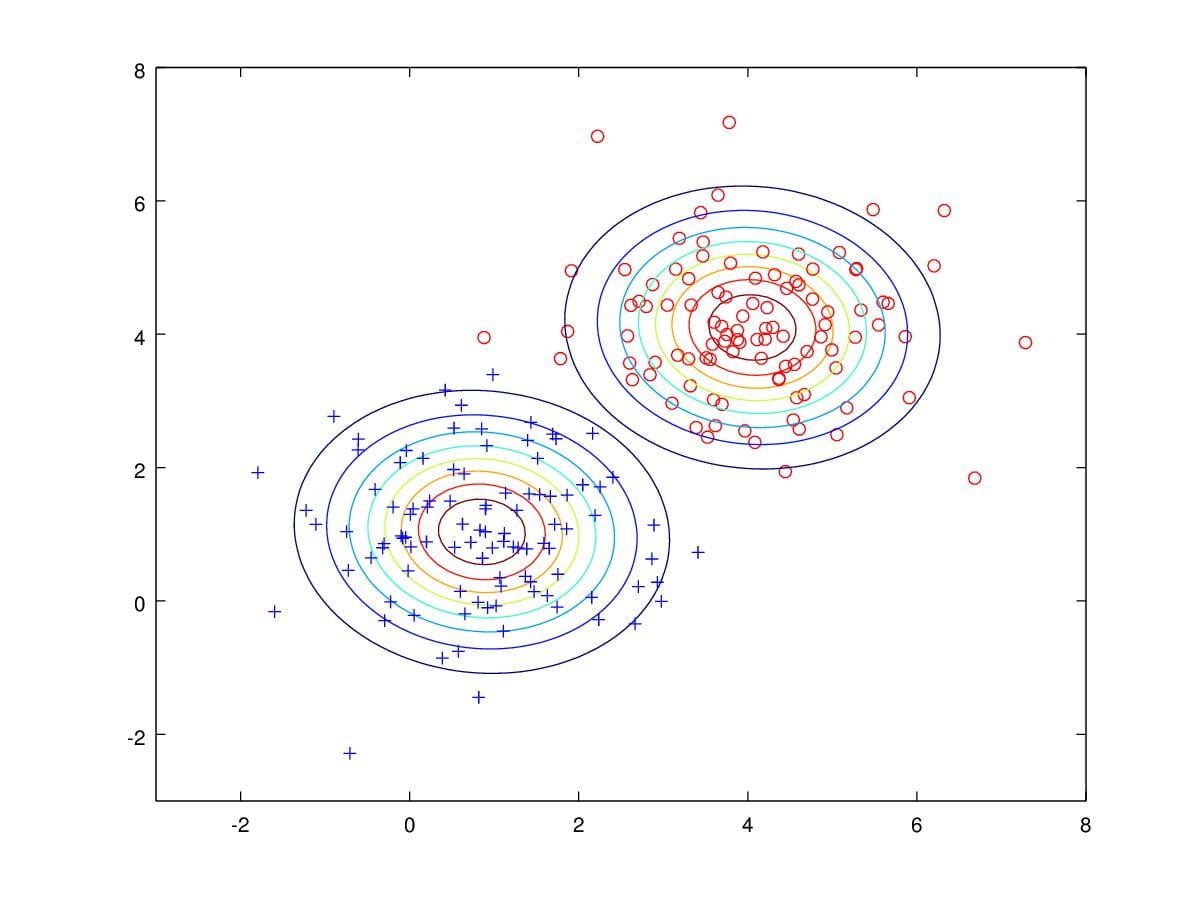
Apply GDA
Notice the data drawn from two Gaussian Distribution is random, thus,
if you run the code, the outcome may be different. However, in most
cases, distributions drawn by estimated parameters are roughly the same
as the original distributions.
[x1 y1]=meshgrid(linspace(-3,8,100)',linspace(-3,8,100)'); X1=[x1(:) y1(:)]; z1=mvnpdf(X1,mu_1,sigma); contour(x1,y1,reshape(z1,100,100),8); hold on; z2=mvnpdf(X1,mu_0,sigma); contour(x1,y1,reshape(z2,100,100),8);
Figure 13. Contours drawn from parameters estimated.
In fact, we can compute the probability of each data point to predict
which distribution it is more likely belongs, for example, if we want to
predict \(x=\begin{pmatrix}0.88007\\3.9501\end{pmatrix}\)
is more of the left distribution or the right, we apply \(x\) to these two distribution:
In light of the equivalency of \(p(y=1)\) and \(p(y=0)\) (both are \(0.5\)), we just compare\(p\left(x=\begin{bmatrix}0.88\\3.95\end{bmatrix}\Bigg|
y=1\right)\) to \(p\left(x=\begin{bmatrix}0.88\\3.95\end{bmatrix}\Bigg|
y=0\right)\). Apparently, this data point is predicted from the
left distribution, which is a wrong assertion. Actually, in this
example, we have only this data pointed classified incorrectly.
You may wonder why there is a blue line. It turns out that all the
data point below the blue line will be considered as blue class.
Otherwise, data points above the line is classified as the red class.
How it work?
The blue line is decision boundary, if we know the expression of this
line, the decision will be made easier. In fact GDA is a linear
classifier, we will prove it later. Still, we see the data point above,
if we just divide one probability to another, we just need find if the
ratio larger or less than 1. For our example, the ratio is roughly 0.68,
so the data point is classified to be the blue class.
Here, \(\mu_1^T\Sigma^{-1}x=x^T\Sigma^{-1}\mu_1\)
because it is a real number. For a real number \(a=a^T\), moreover, \(\Sigma^{-1}\) is symmetric, so \(\Sigma^{-T}=\Sigma^{-1}\). Let's set \(w^T=(\mu_1-\mu_0)^T\Sigma^{-1}\) and \(w_0=-\frac{1}{2}\mu_1^T\Sigma^{-1}\mu_1+\frac{1}{2}\mu_0^T\Sigma^{-1}\mu_0+\log\frac{\phi}{1-\phi}\),
then we have:
If you plug parameters in the formula, you will find:
\(\mathcal{R}=-3.0279x_1-3.1701x_2+15.575=0\)
It is the decision boundary(Figure 14.). Since you have got the
decision boundary formula, it is convenient to use the decision boundary
function predict if a data point \(x\)
belongs to the blue or red class. If \(\mathcal{R}>0\), \(x\in \text{red class}\), otherwise, \(x\in \text{blue class}\).
Conclusion
Today, we have talked about Guassian Distribution and its
Multivariate form. Then, we assume two groups of data drawn from
Gaussian Distributions. We apply Gaussian Discriminant Analysis to the
data. There are 200 data point, only one is misclassified. In fact we
can deduce GDA to Logistic regression Algorithm(LR). But LR can not
deduce GDA, i.e. LR is a better classifier, especially when we do not
know the distribution of the data. However, if you have known that data
is drawn from Gaussian Distribution, GDA is the better choice.
Reference
Andrew Ng http://cs229.stanford.edu/notes/cs229-notes2.pdf


 Since the diffusion map applied the Gaussian kernal during the distances
calculation, it usually a better way to capture the cell differentation
events. Here we show diffusion dimension 1,2 and 1,3. It's clear that
1,2 captures the cell differentation from fibroblasts to neuron, and 1,3
captures the differentiation from firoblasts to myocytes.
Since the diffusion map applied the Gaussian kernal during the distances
calculation, it usually a better way to capture the cell differentation
events. Here we show diffusion dimension 1,2 and 1,3. It's clear that
1,2 captures the cell differentation from fibroblasts to neuron, and 1,3
captures the differentiation from firoblasts to myocytes. 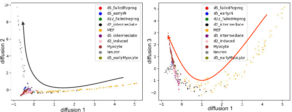
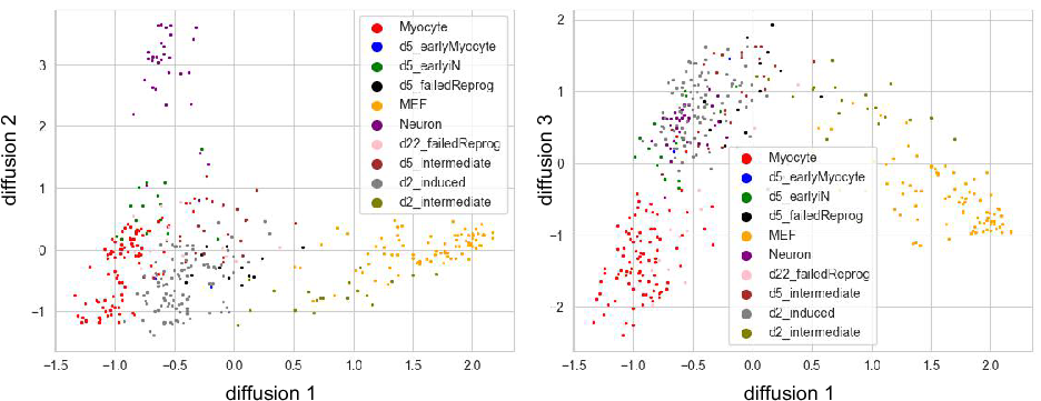
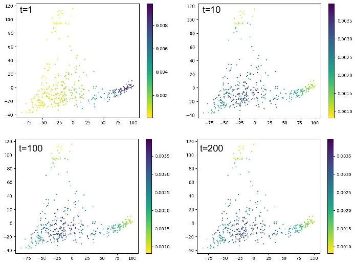
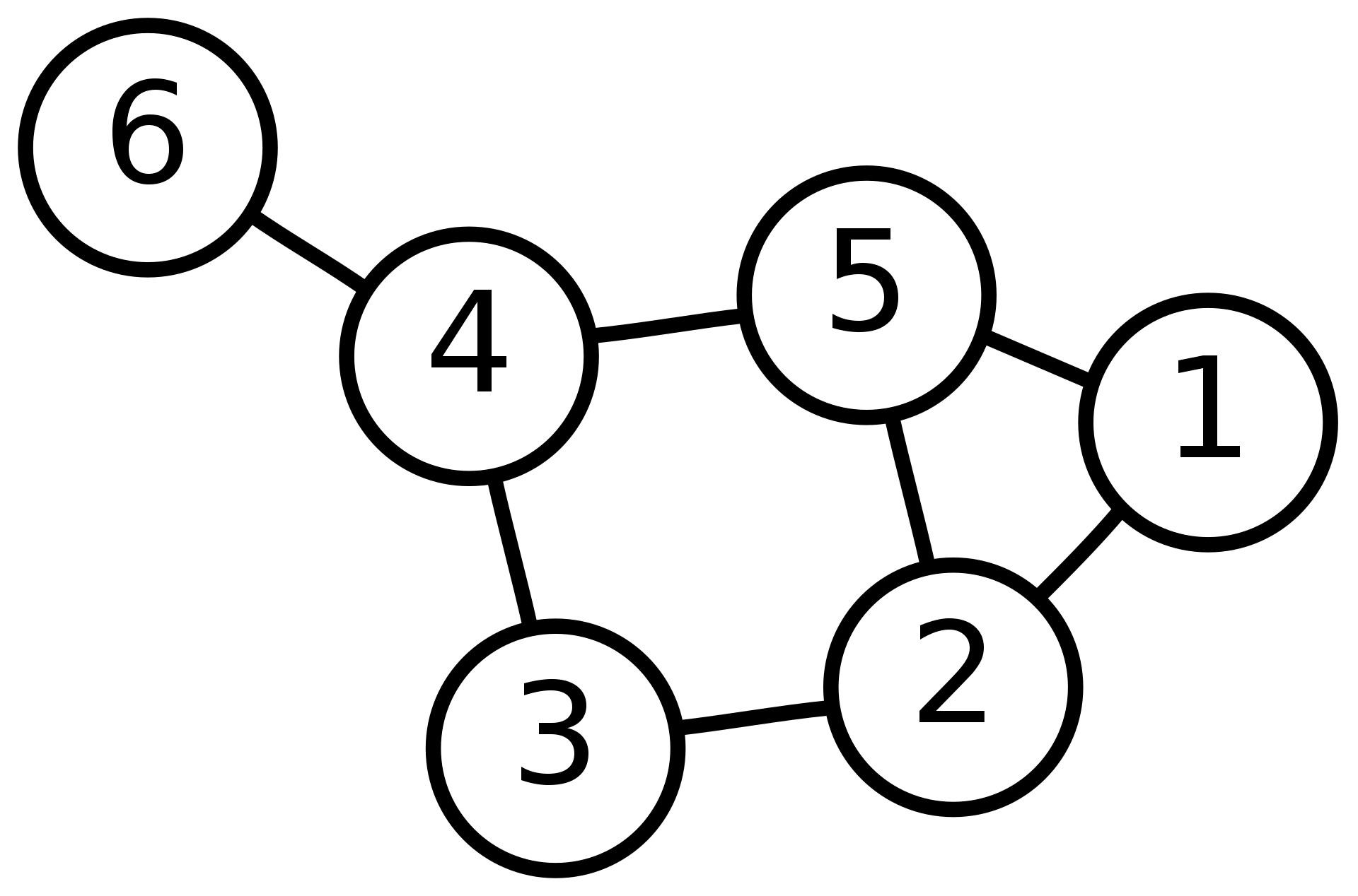
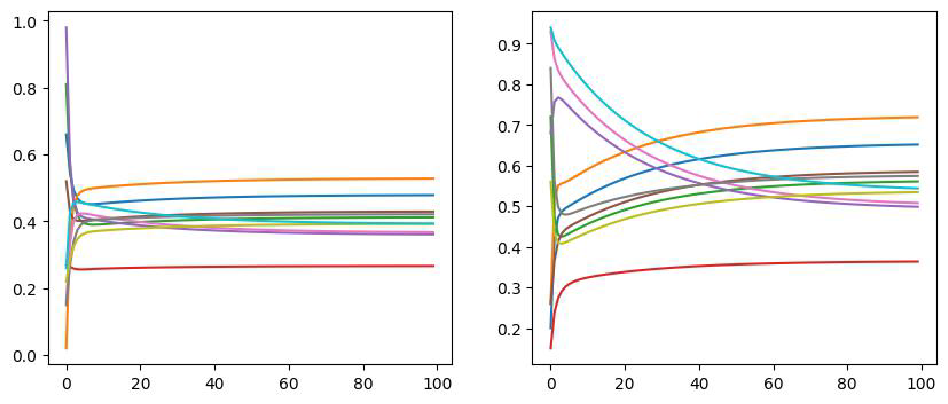
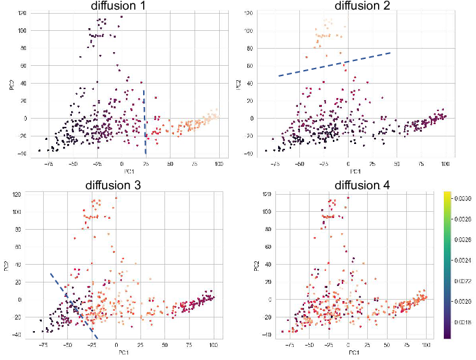
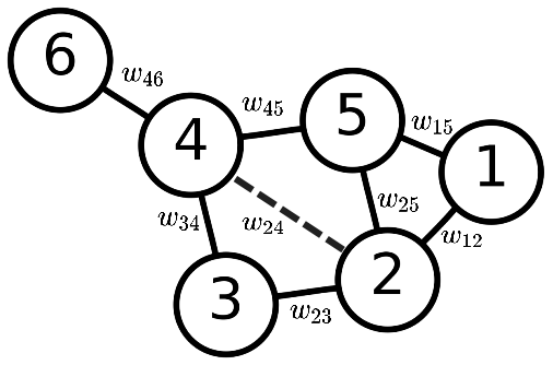
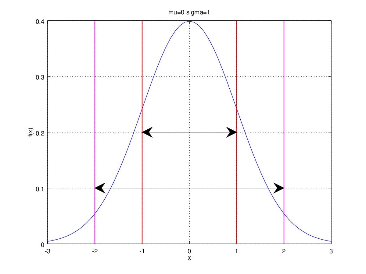 Figure 1. Gaussian Distribution with